Data Fusion for Materials Location Estimation in Construction

Transcription

1 Data Fusion for Materials Location Estimation in Construction by Saiedeh Navabzadeh Razavi A thesis presented to the University of Waterloo in fulfillment of the thesis requirement for the degree of Doctor of Philosophy in Civil Engineering Waterloo, Ontario, Canada, 2010 Saiedeh Navabzadeh Razavi 2010

2 AUTHOR'S DECLARATION I hereby declare that I am the sole author of this thesis. This is a true copy of the thesis, including any required final revisions, as accepted by my examiners. I understand that my thesis may be made electronically available to the public. ii

3 Abstract Effective automated tracking and locating of the thousands of materials on construction sites improves material distribution and project performance and thus has a significant positive impact on construction productivity. Many locating technologies and data sources have therefore been developed, and the deployment of a cost-effective, scalable, and easy-to-implement materials location sensing system at actual construction sites has very recently become both technically and economically feasible. However, considerable opportunity still exists to improve the accuracy, precision, and robustness of such systems. The quest for fundamental methods that can take advantage of the relative strengths of each individual technology and data source motivated this research, which has led to the development of new data fusion methods for improving materials location estimation. In this study a data fusion model is used to generate an integrated solution for the automated identification, location estimation, and relocation detection of construction materials. The developed model is a modified functional data fusion model. Particular attention is paid to noisy environments where low-cost RFID tags are attached to all materials, which are sometimes moved repeatedly around the site. A portion of the work focuses partly on relocation detection because it is closely coupled with location estimation and because it can be used to detect the multi-handling of materials, which is a key indicator of inefficiency. This research has successfully addressed the challenges of fusing data from multiple sources of information in a very noisy and dynamic environment. The results indicate potential for the proposed model to improve location estimation and movement detection as well as to automate the calculation of the incidence of multi-handling. iii

4 Acknowledgements I was privileged to work with Dr. Carl Haas, an exceptional supervisor and a great mentor. I would like to express my sincere appreciation to him for his guidance, encouragement, and support. I am also very grateful for the mentorship and support of Dr. Ralph Haas, Dr. Susan Tighe, and Dr. Frank Saccomanno. In addition, I would like to thank NSERC, the Construction Industry Institute (CII), FIATECH, Ontario Power Generation Inc., SNC-Lavalin, Bechtel, and Identec Solutions for their support of this research. I also acknowledge and thank for their collaboration and helpful advice Dr. Carlos Caldas, Dr. Paul Goodrum, Dr. Francois Caron, Dr. David Grau, Dr. Emmanuel Duflos, Dr. Philippe Vanheeghe, and Dr. Fakhri Karray. The invaluable assistance of my fellow graduate students Duncan Young, Hassan Nasir, and Bahador Khaleghi and of other graduate and undergraduate students, who collaborated on publications and/or contributed to the field implementation, is also deeply appreciated. iv

5 Table of Contents AUTHOR'S DECLARATION... ii Abstract... iii Acknowledgements... iv Table of Contents... v List of Figures... xi List of Tables... xv Chapter 1 Introduction Background and Motivation Research Objectives Research Scope Research Methodology Thesis Organization... 8 Chapter 2 Background and Literature Review Construction Site Materials Management Current site Materials Handling Process Automated Materials Management Systems and Technologies RFID Applications in Construction Applications of GPS in Construction Building Information Modeling Multisensor Data Fusion The Benefits of Multisensor Data Fusion Multisensor Data Fusion Algorithms Data Fusion Models Multisensor Data Fusion Challenges Multisensor Data Fusion Applications Wireless sensor networks and Sensor Network Localization Sensor Network Location Estimation Methods Context and Context-Aware Systems The Knowledge Gap Chapter 3 Field Implementation and Data Acquisition Framework Data Acquisition Framework and the Integrated Technology v

6 3.2 Uncertainties and Imprecision Due to the Limitations of the Physical Components Preliminary Field Experiments at the University of Waterloo Objectives Obstructing Materials Test for RFID Post-Processing GPS Precision Test Circular Proximity Test for RFID Read Range Reliability Field Experiments at Industrial Construction Job Sites Objectives Portlands Energy Centre Field Trials Field Experiments in Rockdale, Texas Impacts of the Field Trials and Experiments Acquired Data Set Control Experiments Summary Chapter 4 Data Fusion Model and Evaluation Metrics Data Fusion Model and Architecture Data Fusion Level Data Fusion Level Data Fusion Level Data Fusion Levels 3, 4 and Human/Computer Interaction BIM Data Fusion Implementation Data Fusion Model Evaluation Metrics Summary Chapter 5 Data Fusion Levels 0 and 1: Reliability-Based Location Estimation Data Fusion-Level 0: Sensor Reliability Detection Why Fuzzy? Fuzzy Inference System Input Variables Fuzzy Inference System Output Variables Fuzzy Inference Rules Defuzzification Data Fusion-Level 1: Hybrid Location estimation vi

7 5.2.1 The Dempster-Shafer Theory for Hybrid Location estimation Hybrid Weighted Averaging Field Experiment Setup Portlands Trial Data Subset Control Experiment Data Subset Experimental Results Performance Measurement of the Control Experiment Performance Measurement of the Portlands Experiment Summary Chapter Data Fusion-Level 2: Relocation Detection Dempster-Shafer theory for Detecting Relocation Field Experiment Setup Portlands Trial Data Subset Control Experiment Data Subset Experimental Results Performance Measurement of the Portlands Experiment Performance Measurement of the Control Experiment Summary Chapter 7 Conclusions and Future work Conclusions Contributions Limitations Outlook and Future Work Bibliography Appendices Appendix A Principles of Radio Frequency Identification Technology Appendix B Principles of Global Positioning System Appendix C Belief Function Theory: An Overview and the Implementation Model Appendix D Benefit Cost Model for RFID/GPS Based Automated Materials Tracking System Appendix E A Sample Subset of the Acquired Data from the Filed Experiment Appendix F Implementation Document for the Software in Visual C#.NET vii

8 Table of Contents Namespace Index I. Package List Class Index II. Class List Namespace Documentation III. Package RFID_GPS_LocationSensing_Project i Packages ii Classes IV. Package RFID_GPS_LocationSensing_Project.Properties iii Classes Class Documentation V. RFID_GPS_LocationSensing_Project.ReadEvent Class Reference iv Classes v Public Member Functions vi Properties vii Private Member Functions viii Static Private Member Functions ix Private Attributes x Detailed Description xi Member Function Documentation xii Member Data Documentation xiii Property Documentation VI. RFID_GPS_LocationSensing_Project.FinalTagLocation Class Reference xiv Public Member Functions xv Public Attributes xvi Properties xvii Static Private Member Functions xviii Private Attributes xix Detailed Description xx Member Function Documentation xxi Member Data Documentation viii

9 xxii Property Documentation VII. RFID_GPS_LocationSensing_Project.Form1 Class Reference xxiii Public Member Functions xxiv Private Member Functions xxv Detailed Description xxvi Constructor & Destructor Documentation xxvii Member Function Documentation VIII. RFID_GPS_LocationSensing_Project.GPSData Class Reference xxviii Public Member Functions xxix Properties xxx Detailed Description xxxi Member Function Documentation xxxii Property Documentation IX. RFID_GPS_LocationSensing_Project.Program Class Reference xxxiii Static Private Member Functions xxxiv Detailed Description xxxv Member Function Documentation X. RFID_GPS_LocationSensing_Project.ReadEvent.Ellipsoid Class Reference xxxvi Public Member Functions xxxvii Public Attributes xxxviii Detailed Description xxxix Constructor & Destructor Documentation xl Member Data Documentation XI. RFID_GPS_LocationSensing_Project.Properties.Resources Class Reference xli Properties xlii Private Member Functions xliii Static Private Attributes xliv Detailed Description Constructor & Destructor Documentation xlv Member Data Documentation xlvi Property Documentation ix

10 xlvii internal global::system.resources.resourcemanager RFID_GPS_LocationSensing_Project.Properties.Resources.ResourceManager [static, get, private] XII. RFID_GPS_LocationSensing_Project.RFID_TAG Class Reference xlviii Public Member Functions xlix Properties l Detailed Description li Member Function Documentation lii Property Documentation XIII. RFID_GPS_LocationSensing_Project.Properties.Settings Class Reference liii Properties liv Static Private Attributes lv Detailed Description lvi Member Data Documentation lvii Property Documentation x

11 List of Figures Figure 1.1: Research Methodology... 6 Figure 2.1: Structure of the literature review for the thesis... 9 Figure 2.2: (Con)fusion of terminology (Steinberg, 2001) Figure 2.3: Revised JDL data fusion model (Steinberg, 1998) Figure 2.4: Data fusion waterfall model (adapted from Esteban (2005)) Figure 2.5: Data fusion waterfall model (adapted from Esteban (2005)) Figure 2.6: Lateration and angulation Figure 2.7.: Localization based on time difference of arrival (Krishnamachari 2005) Figure 2.8: Evolution of the pignistic probability of each cell as a function of new reads Figure 2.9: Modeling the RF communication region under the occupancy cell framework (Song 2005) Figure 2.10: Illustration of the functioning of proximity methods Figure 2.11: Accumulation of cell magnitude after each read using the accumulation array method, with a discrete read range of ρ= Figure 3.1: System network diagram Figure 3.2: Material tracking technologies used for the research Figure 3.3: System physical components and their relationships Figure 3.4: GPS with sub-foot accuracy in post-processing Figure 3.5: GPS data from a sample gridded field before (left side) and after (right side) the differential correction was performed Figure 3.6: The short read range reliability test results for the active RFID tags (distances are in meters) Figure 3.7: The long read range reliability test results for the active RFID tags (distances are in meters) Figure 3.8: The construction site layout (Photo source: The project website and Google map) Figure 3.9: Tagged pipe spools at the receiving point Figure 3.10: Field trial procedure Figure 3.11: (a) Pipe spools at site lay-down areas (b) Pipe spools at the port Figure 3.12: A sample of tagged pipe spools Figure 3.13: Sample maps with different scales, showing RFID tag locations Figure 3.14: Illustration of the data fields of a sample.kml file xi

12 Figure 3.15: Controlled Field experiment in a parking lot Figure 3.16: Georeferenced plan of the deployment of the tags into separate blocks Figure 3.17: Sample results of logging the locations of the tags Figure 4.1: Data fusion model for construction resource location estimation Figure 4.2: Hierarchical relationship representation among read events, observations, and the improved location estimation through data fusion Figure 4.3: The effect of relocation detection on the expected localization error Figure 4.4: UML Component diagram for a high-level view of the system Figure 4.5: Schematic representation of the observations and estimation methods used in the fusion level 1 for n pairs of observed locations Figure 4.6: Schematic representation of accuracy and precision Figure 5.1: Fuzzy contextual variable: PDOP Figure 5.2: Fuzzy contextual variable: RSSI Figure 5.3: Fuzzy contextual variable: GPS accuracy Figure 5.4: Fuzzy contextual variable: location relative to the lay-down yard Figure 5.5: Reliability degree as the fuzzy output Figure 5.6: Fuzzy inference rules engine Figure 5.7: Sample of firing fuzzy inference rules for the input set of [ ] Figure 5.8: Sample of firing fuzzy inference rules for the input set of [ ] Figure 5.9: Discrete frame of discernment and modeling the RF communication region Figure 5.10: The proposed solution mass allocation Figure 5.11: Scatter chart for the true value (red point) and the measurements (blue points) of the tag ID (a) The original values (b) Values shifted toward the origin Figure 5.12: Portlands trial: Scatter plot of sample observations after biasing them all to the centre. 93 Figure 5.13: Control experiment: Scatter plot of sample observations after biasing them all to the centre Figure 5.14: Portlands trial: Original location error distribution in the observed sample subset Figure 5.15: Two samples of the identification of components outside the boundaries for real locations (BIM) Figure 5.16: Control experiment: Original location error distribution in the observed sample data subset xii

13 Figure 5.17: Sample data with some of the observations having a relative location outside the allowed boundaries (BIM) Figure 5.18: Control experiment - scatter plot for: (left-top) benchmarks (right-top) original observations (left-middle) 18 Centroid estimates per tag (right-middle)18 hybrid weighted averaging estimates per tag (left-bottom) 18 Dempster-Shafer estimates per tag (right-bottom)18 hybrid Dempster-Shafer estimates per tag Figure 5.19: Control experiment Mean of absolute error for different localization methods Figure 5.20: Control experiment- Standard deviation of absolute error for different localization methods Table 5.6: Control experiment Absolute error distribution parameters for the last observation of each tag; obtained for 10 different random input data sets Figure 5.21: Control experiment A comparison of the absolute error distribution parameters for the final observation of different fusion algorithms Figure 5.22: Portlands trial Mean of absolute error for different localization methods, original acquired data with no simulation Figure 5.23: Portlands trial Standard deviation of absolute error for different localization methods, original acquired data with no simulation Figure 5.24: Comparing the field experiments for mean of absolute error of different algorithms Figure 5.25: Comparing the experiments in terms of standard deviation of absolute error of different algorithms Figure 5.26: Portlands trial Mean of absolute error for different localization methods, simulated PDOP and corrupted coordinates with normal error of mu=4 and sigma= Figure 5.27: Portlands trial Standard deviation of absolute error for different localization methods, simulated PDOP and corrupted coordinates with normal error of mu=4 and sigma= Figure 5.28: Portlands trial Mean of absolute error for different localization methods, simulated PDOP and corrupted coordinates with normal error of mu=10 and sigma= Figure 5.29: Portlands trial Standard deviation of absolute error for different localization methods, simulated PDOP and corrupted coordinates with normal error of mu=10 and sigma= Figure 5.30: Portlands trial Mean of absolute error for different localization methods, simulated PDOP and corrupted coordinates with normal error of mu=20 and sigma= Figure 5.31: Portlands trial Standard deviation of absolute error for different localization methods, simulated PDOP and corrupted coordinates with normal error of mu=20 and sigma= xiii

14 Figure 6.1: Location error distribution of all the observations in the data subset Figure 6.3: Receiver Operating Characteristic Curve (ROC) for different conflict thresholds Figure 6.4: Receiver Operating Characteristic Curve (ROC) for different hypothetical read ranges 120 Figure 6.5: Distribution of the distance between benchmark locations of all dislocated sample as opposed to true-positive detections, for conflict-threshold = 0.8 and hypothetical read range=16m. 120 Figure 6.7: ROC curves for different values of the basic belief assignment and different ratio between the focal elements Figure 6.8: ROC curves for different values of the basic belief assignment and the same ratio between the focal elements (2 to 1) Figure A.1: Schematic RFID-based system framework Figure B.1: Differential GPS positioning Figure E.1: Illustration of the data fields of a sample.kml file xiv

15 List of Tables Table 2.1: Benefits of Multisensor Data Fusion (Walts, 1986) Table 2.2: Data Fusion Methodologies Table 2.3: Representative multisensory data fusion applications Table 3.1: Results of the obstructing materials test Table 5.1: DOP values for GPS signal reliability verification (Binary Logic) Table 5.2: Control experiment Mean of absolute error for different localization methods (Algorithms bias) Table 5.3: Control experiment- Standard deviation of absolute error for different localization methods Table 5.4: Control experiment Means of absolute errors for the last observation; obtained for 10 different random input data set Table 5.5: Control experiment Standard deviation of absolute errors for the last observation; obtained for 10 different random input data sets Table 5.7: Portlands trial Mean of absolute error for different localization methods, original acquired data with no simulation Table 5.8: Portlands trial Standard deviation of absolute error for different localization methods, original acquired data with no simulation Table 5.9: Portlands trial Mean of absolute error for different localization methods, simulated PDOP and corrupted coordinates with normal error of mu=4 and sigma= Table 5.10: Portlands trial Standard deviation of absolute error for different localization methods, simulated PDOP and corrupted coordinates with normal error of mu=4 and sigma= Table 5.11: Portlands trial Mean of absolute error for different localization methods, simulated PDOP and corrupted coordinates with normal error of mu=10 and sigma= Table 5.12: Portlands trial Standard deviation of absolute error for different localization methods, simulated PDOP and corrupted coordinates with normal error of mu=10 and sigma= Table 5.13: Portlands trial Mean of absolute error for different localization methods, simulated PDOP and corrupted coordinates with normal error of mu=20 and sigma= Table 5.14: Portlands trial Standard deviation of absolute error for different localization methods, simulated PDOP and corrupted coordinates with normal error of mu=20 and sigma= Table 6.1: Relocation detection rate with respect to conflict threshold xv

16 Table 6.2: Relocation detection rate with respect to the hypothetical read range (Conflict threshold = 0.4) Table D.1: Benefit Cost Model for RFID/GPS based automated materials tracking system xvi

17 Chapter 1 Introduction 1.1 Background and Motivation In industrial and heavy construction, as prefabricated objects such as pipe spools and precast concrete elements are assembled and installed on site, the designed facilit takes shape, and its progress can be tracked. Decreasing the occurrence of unsuccessful searches for the required materials reduces the amount of supervisory time wasted, the amount of idle time for the crew, and the number of disruptions to short-interval planning. Concomitantly, understanding the flow of materials over time helps to increase labour productivity, reduces the stockpiling of materials, and decreases the manpower required for materials management (Bell and Stuckhart, 1986). On a large construction site, achieving these goals can involve locating and tracking tens of thousands of critical units of materials. Effective site materials management can address the problem of unsuccessful searches and also contribute significantly to the success of a project. An optimized materials management system can increase productivity, help avoid delays, reduce the number of man hours needed for materials management, and lower expenditures for materials by decreasing waste. Such a system on a site can ensure that sufficient quantities of materials and equipment are available for construction needs and that surplus at the end of the project is minimized. It can also have a significant effect on the project schedule (Thomas 2000). Materials tracking and locating technologies are key elements in optimized materials management systems. Deficiencies in materials management have been recognized by Thomas et al. (1992) as the most significant and common factor affecting construction productivity and have been estimated by Nasir et al. (2009) to cause an overall reduction in productivity of up to 40 %. Late deliveries, rehandling and misplacement of components, incorrect installation, and other problems intrinsic to the existing manual methods of locating highly customized materials can lead to delays in the project schedule and increases in labour costs (Ergen, 2007). While automated controls are often established for engineered and other critical materials during the design and procurement stages of large industrial projects, typical on-site control practices are still based on direct human observation, manual data entry, and adherence to processes. These methods do not adequately overcome the dynamic and unpredictable nature of construction sites, and the resulting unavailability of construction materials at the right place and at the right time 1

18 has been recognized as having a major negative impact on productivity. Moreover, poor site materials management potentially delays construction activities and thus threatens project completion dates, which is likely to increase the total installed costs (Grau, 2007a). An accurate and automated site materials management system that can identify and localize the materials both on the site and further up the supply chain will therefore have a significant positive effect on the materials control problem and associated shortages and can also facilitate automated material receiving and inventory control. In an initial attempt to automate materials tracking, Caldas et al. (2006) implemented a mapping approach based on Global Positioning System (GPS) and handheld Geographic Information System (GIS) that demonstrated some promise for time savings and reduced materials losses under specific conditions. In this study GPS was used to record the position of pipe spools on an industrial construction project. Although this approach may seem an obvious solution for locating and tracking the construction materials but attaching a GPS receiver to each construction material is expensive and is not a viable option for large scale implementation on construction sites. In addition to economical limitations, this approach has a number of other significant limitations such as GPS signal blockage due to the orientation of the GPS tags and the high density materials and surrounding structures. Specific examples of more recent research are demonstrating that, coupled with mobile computers, data collection technologies and sensors can provide cost-effective, scalable, and easy-to-implement materials location sensing at actual construction sites (Akinci, 2002; Song, 2006a; Song, 2006b; Caldas, 2006; Grau, 2007;, Teizer, 2007; Razavi, 2008; El-Omari, 2009). One of these examples is the study by Ergen et al. that used a crane-mounted GPS receiver to track the discrete movements of the RFID-tagged precast concrete materials on the staging yard (Ergen 2007). The results of this study show that 60% of relocated materials were detected correctly. More sophisticated and automated data collection technologies based on wireless sensor networks that use GPS and RFID (Radio Frequency Identification) are being developed for a wide spectrum of applications. A cost-benefit analysis for RFID/GPS Based automated materials tracking system presented in Appendix D of this thesis shows the significant benefits of utilizing this integrated solution for locating materials in construction site (Nasir 2009). Although a number of successful studies have attempted on the application of automated sensing technologies for construction materials localization, but some important areas were still untouched. While most of these studies were conducted in small-scale ideal-condition 2

19 experiments, the feasibility of applying these approaches in a fully automated manner is a realworld construction job site was yet to explore. In 2008, Grau et al. presented a comprehensive study and field experiments that were partly conducted in collaboration with the author s current research study (Grau 2008, Grau 2009, Razavi 2008). Grau et al. assessed and quantified the impact of the integrated solution of RFID and GPS for automatically tracking the materials in real-world construction projects. In this study, two localization techniques of Centroid and a constrained-based technique based on proximity have also been explored and compared to estimate the components locations. Results show that Centroid model presents higher performance compare to the proximity methods. These techniques have been used in this thesis to provide a benchmark for comparing different localization methods in different conditions. A key challenge is to find ways of improving the performance of the above-mentioned methods while maintaining the cost-effectiveness and scalability. Also with rapid advances in sensing technologies, having a method that can be robust to future advances of technology and also be sensitive to materials relocation is another important challenge. To address this challenge, this research has developed a data fusion model that provides an integrated solution for automated identification, location estimation, and relocation detection of construction materials. The developed model is a modified functional data fusion model. A critical element of this framework is the location estimation problem; developing a data fusion method for location estimation that is robust with respect to measurement noise while having a reasonable implementation cost would therefore be advantageous. Fusing a variety of sources of location and contextual data, such as building information modeling (BIM), is intended to increase confidence, achieve better performance for location estimation, and add robustness to operational performance. Particular attention has been paid to relocation detection because it is closely coupled with location estimation and because it can be used to detect multi-handling of materials, which is a key indicator of inefficiency. The focus of this thesis is therefore on the location estimation and relocation detection problems and on the potential of data fusion to solve these problems. 1.2 Research Objectives To address the above mentioned challenges, sensors ranging from simple to complex can be utilized: RFID transponders, GPS receivers, RFID readers, RFID with GPS chips, UWB, ultrasound, infrared, and others. It is assumed that a small subset of sensors will have a priori information about their locations because they have been coupled with GPS receivers or GPS 3

20 chips, or because they have been installed at fixed points with known coordinates. This subset is small because no matter how a priori location information is acquired, it is on average one or two magnitudes more expensive per sensor node than estimated location information. For example, many geomatics solutions exist for tracking items accurately and in real time but at a cost that is prohibitive for the problem described here. In addition, even sophisticated and expensive solutions experience, to some extent, multipath, dead space, and environmentally related interference. Thus, developing a method for location estimation that is robust with respect to measurement noise while having a reasonable implementation cost is a challenge. One promising approach is to use data fusion. Data fusion is defined as the process of combining data or information in order to estimate the state of an entity. In most cases, the state of an entity refers to a physical state, such as identity, location, or motion over a period of time; in this case, it refers to the location of a construction material. Given these factors, the objective of the proposed research is therefore to develop a more accurate and reliable location estimation method based on data fusion that is robust to measurement noise and to future advances in technologies, scalable to tens of thousands of items, and effective enough to be used for automated identification of dislocated materials. Field experiments were used to validate the model; to demonstrate the feasibility of employing the components, methods, and technologies developed; and to facilitate the deployment of the technology and its transfer to industry. These experiments have been underway for three years. In summary, the hypothesis to be examined is that data fusion can improve location estimation on construction sites and help with the detection of locations and relocations. 1.3 Research Scope This research study was conducted within the following outlined scope: Materials location but not the location of people or equipment Stationary objects that are subject to discrete shifts in location Very large projects with many critical materials (typically >5,000 items) such as valves, pipe spools, structural steel, etc. Methods suitable for very noisy, dynamic environments Exploitation of existing or soon-to-be-existing data sources 4

21 1.4 Research Methodology The research began with a problem statement and the definition of the preliminary scope and objectives. These led to a comprehensive literature review, which covered a wide spectrum of related information, including studies related to multisensor data fusion, wireless sensor networks and sensor network localization, construction site materials management, automated material management systems and technologies, building information modeling, and context and context aware systems. While initial field trials were being conducted, the data fusion architecture and algorithms were also gradually designed. Computational experiments for implementing the algorithms and integrating them with the existing devices and technologies were then conducted. Field trials were performed at a construction site and were continued in order to assess the feasibility of utilizing this approach in the real world. Other control experiments were also conducted to support the results obtained from the real-world implementation. Fusion model levels 0, 1, and 2 were validated using the data acquired from the real-world trial as well as from the control experiments. Finally, all the knowledge, experiments, and lessons learned were documented and presented along with recommendations for further work. Figure 1.1 shows schematically the research methodology outlined and defined as follows: Problem statement: Identify the existing needs and problems in order to define the research idea, objectives, and main scope. Literature review. Design of the data fusion algorithm and architecture: The data fusion model and the algorithms at the various levels of the model as well as the approaches used for the functional levels were designed. The approaches for fusing the data include a JDL fusion model adapted for the application in this research; Dempster-Shafer evidence-based reasoning, hybrid Dempster-Shafer, Centroid, and hybrid weighted averaging methods for location estimation; a fuzzy logic inference engine; a Dempster-Shafer algorithm for relocation detection; and a validation method. Implementation of the algorithms: The algorithms designed for the functional data fusion levels required implementation software that would also integrate them with the sensing technologies. 5

22 Research Methodology Data Fusion for Location Estimation in Construction Preliminary Stage Problem Statement Literature Review Design and Implementation Algorithms Implementation Design Data Fusion Algorithms and Architechture Technology Integration Field Trial Field Trial Field Data Evaluation Analysis of Field Data to Validate the Fusion Model Conclusion and Documentation Conclusion and Recommendation Documentation Periodic Reports, Papers and PhD thesis Figure 1.1: Research Methodology Technology integration: In this step, the existing physical and developed functional componentswere integrated, which included the identification of the communication scenarios of the components, such as GPS, RFID, handheld PC, wireless communication, and GIS navigation, as well as the development of the data visualization technique. The challenges associated with the practical integration of the developed software within the framework were also addressed at this stage. 6

23 Field trials: Field trials were conducted at a variety of levels. o o o Most of the new developments were first tested in the lab. Then small-scale field trials took place on the University of Waterloo (UW) campus before field trials were attempted at the partners facilities. Additional small-scale experiments on campus were also conducted. Two industrial pilot projects then hosted the field trials, which were conducted at sites in Toronto and Texas, providing an opportunity to test the developed system. After the experiments were conducted, data were collected, and the results were reported to site management. The trials required collaboration with partners so that the experimental plans could be detailed for the host projects; SNC Lavalin, OPG, and Identec Solutions supported this work. At the Portlands site in Toronto, critical components such as valves, pipe spools, and pipe supports were tracked. In other similar trials in Rockdale, Texas, structural steel was the target of the tracking. The first step in the field trials was to analyze both the current process of handling the materials on the site and the information flow for the project. The critical components to be tracked were then selected, the field trial scenario was designed, and the data collection procedures were developed with the collaboration of SNC Lavalin s site management personnel. The system was then deployed, maps were produced, and the data were collected. A simple control experiment was conducted on a parking lot on campus in order to acquire a more controlled version of the data set. Analysis of field data to validate fusion model: To test the flexibility and power of the fusion model, the validating procedure included a variety of sets of experiments and data sets. The data collected from the real-world construction site trial and from the control experiments were used to run and validate the fusion model. The daily logged data of all the sensed information and the existing contextual data constitute the input for the model. Location data logs from a high-accuracy GPS are used to validate the output of the model, which is comprised of the estimated locations of the tagged construction resources as computed by the model. Conclusions and Documentation. 7

24 1.5 Thesis Organization This thesis is organized in six chapters. Chapter One provides an overview of the research problem and describes the motivation, objectives, scope, and methodology of the research. Chapter Two provides background knowledge about multisensor data fusion, wireless sensor networks, sensor network localization, construction site materials management, automated materials management systems and technologies, building information modeling, and context and context aware systems. Chapter Three presents the field implementation and data acquisition framework for the automated construction materials tracking system. The data fusion model and the details of the development are presented in chapter Four. Chapter Five discusses the fusion levels 0 and 1 toward the objective of materials location detection and Chapter Six presents the fusion 2 for relocation detection. Chapter Seven summarizes the proposed research and presents possibilities for future work. 8

25 Chapter 2 Background and Literature Review This thesis presents research that addresses problems in the management of construction site materials by developing an integrated solution framework. This integrated solution builds on some of the technologies, methods, and concepts used in automated materials management, wireless sensor network localization, data fusion, and building information modeling. A review of the basic concepts of these areas and related prior studies is provided in this chapter. Figure 2.1 schematically presents the architecture of the background studies required. Figure 2.1: Structure of the literature review for the thesis 2.1 Construction Site Materials Management This research effort was inspired by the studies that showed effective construction site materials management systems have significant impact on construction productivity (Bell 1986, Thomas 1989, and Thomas 2000). Materials management encompasses storage, identification, retrieval, transport, and construction methods (Thomas, 2002). According to the CII materials management handbook (1999), project materials are categorized into three groups that require different approaches during the planning and construction phase: 9

26 Engineered materials: These are items with a unique identification number so that they can be uniquely identified during the project life cycle. Some of these materials, such as tanks and pumps, are engineered or fabricated specifically for the project while others are manufactured according to industry-wide specifications and are also uniquely tagged for control purposes. Valves are an example of the latter type of equipment. Bulk materials: These items are manufactured according to industry standards and are usually purchased in large quantities, such as pipes, cables, and wiring. Prefabricated materials: These materials are fabricated according to engineering specifications at a fabrication shop or at a site separate from the construction site. Structural steel, pipe spools, ladders, and platforms are examples of prefabricated materials. Effective site materials management of all three of the above types of materials can significantly contribute to the success of a project. According to the CII materials management handbook (1999), materials management is one of the most controllable factors that affect craft productivity, and construction schedule. To be effective, however, the site materials management activities must be a fundamental part of an overall materials management program. An effective materials management system has significant impact on the areas such as craft labor hours, number of site materials management personnel, administrative costs for tracking expenditures and budgeting, surplus, the risk of schedule delays, and many others. An optimized materials control system on the site can ensure that the sufficient quantities of materials and equipment are available for construction needs and that surplus at the end of project is minimized. This optimized system can also have a significant effect on the project schedule (Thomas 2000). Deficiencies in materials management have been recognized by Thomas et al. (1992) as the most significant and common factor affecting construction productivity and have been estimated by Nasir (2009) to cause an overall reduction of about 40 %. These deficiencies often occur due to one or more of the following factors (CII Materials Management Handbook 1999, Thomas 1992): Lost or damaged materials Multiple handling of materials Materials required but not purchased Materials purchased but not received 10

27 Sporadic and out-of-sequence deliveries Errors in the material takeoff Variances for additional material requirements Materials that are issued to crafts and are then not used or installed In a seminal paper, Bell and Stukhart (1986) identified the attributes of materials management systems on large and complex industrial construction projects to include the functions of quantity takeoff, vendor evaluation, purchasing, expediting, receiving, warehousing, and distribution. Bell and Stukhart (1987) also quantified the costs and benefits of materials management systems and concluded that an effective materials management system could reduce typical surpluses of bulk materials from 5-10% down to about 1-3% of the bulk materials purchased. Their research showed that on projects where there is a lack or absence of a materials management system, craft foremen spend up to 20% of their time searching for materials and another 10% tracking purchase orders (POs) and expediting. Thomas et al. (1989) studied the impact of materials management on labor productivity. Their case study on medium sized commercial construction projects showed a benefit/cost ratio of 5.7/1.0 for effective materials management. Adverse materials management conditions were identified which include: extensive multiple handling of materials, materials improperly sorted or marked, running out of materials, and crew slowdowns in anticipation of material shortages. Akintoye (1995) estimated that an efficient materials management and control system could potentially increase productivity by 8%. This increase in productivity is mainly attributed to the availability of the right materials prior to the commencement of work and the ability to better plan the work activities due to availability of materials. Choo et al. (1999) found that the biggest problem faced by the field workers is dealing with discrepancies between the anticipated, actually needed and available resources, which include materials. Thomas and Sanvido (2000) examined three case studies of subcontractor-fabricator relations. Their research concluded that inefficient materials management could lead to an increase in field labor hours of 50% or more. Recent analysis of the Construction Industry Institute s Benchmarking and Metrics program s data corroborates these results (CII 2009). In summary, an efficient materials management system can increase productivity, avoid delays, reduce hours needed for materials management, and reduce the cost of materials due to decrease in wastage. Implementation of conventional materials management practices continues to vary widely, however, and this variability and the inability to handle exceptional circumstances such as snow cover and congested delivery patterns limits their potential to improve project 11

28 performance, thus attention is increasingly becoming more focused on the automation of at least some aspects of materials management. Late deliveries, re-handling and misplacement of components, incorrect installation, and other problems inherent in the existing manual methods of locating highly customized materials can lead to delays in the project schedule and increases in labour costs (Ergen 2007). Having an accurate and automated site materials management system that can identify and localize the materials both on the site and further up the supply chain can have a significant positive effect on the materials control problem and associated shortages and can also facilitate automated material receiving and inventory control. The next section discusses these automated site materials management systems and technologies, with a particular attention to the technologies used in this research effort Current site Materials Handling Process Effective site materials management tasks are defined beyond the activities of receiving, storing, and distributing materials. Personnel assignment, materials control, field procurement, field warehousing and craft labor planning comprise a significant part of the site materials management tasks (CII 1999). Grau et al. (Grau 2006) describes the current materials locating process based on KBR`s onshore operations for handing pipe spools on industrial project. The process begins by receiving materials from the manufacturers and continues until materials are distributed to contractors. This includes receiving, unloading, sorting, storing, recalling and loading the materials. Laydowns are divided in grids of approximately m. Receiving: On-site warehouse personnel receive materials that are marked with its unique identification code. During the receiving process, materials are unloaded in predefined areas without identifying or classifying them. The received items are recorded manually into the project management system based on the packing list. This database will further be used for the availability of the materials on site. Sorting: Warehouse personnel sort the materials based on their category, physical characteristics, and identification codes. Sorting and grouping is usually marked down with colored tapes. Then material`s unique ID, grid, and color code are entered manually into the materials management system. This phase is very labor intensive but helps to facilitate the retrieving process. 12

29 Storing: Usually materials will remain in the same grid as they have been received and sorted. However, they may be moved to facilitate the retrieval of an adjacent material. If this moving causes a change in the grid number of the stored material, then the new grid information should be recorded and updated in the system. Recalling: When a specific material is recalled, its grid location and color code is retrieved based on the material`s identification code. Then the craft labors try to visually locate the material in the grid. Because of the visual similarities of many of items, sometimes they need to study the drawings and descriptions of the materials to more easily detect the component. Once an item is located, a flag is attached to assist and facilitate the loading process. Loading: At a predefined schedule, all flagged materials are picked up, loaded, and released to the contractors for installation or pre-assembly. 2.2 Automated Materials Management Systems and Technologies Automated materials management systems can provide the communication and information tools required for efficient identification, inventory, locating, and tracking of goods as well as the reporting and control of their transport to shops and job sites. On large projects, it has been stated that proper reporting and control can usually be achieved by a fully integrated materials management system (CII 1999). The main aim of using ADC technologies in construction is to increase efficiency, reduce data entry errors caused by human transcription, reduce bottlenecks, and reduce labor costs. Such a system is generally comprised of integrated computer hardware, software, and middleware that identify and track the materials and report on and facilitate their control. The scope of these systems ranges from quantity takeoff through materials control and procurement to the construction and startup phases of a project. Tracking the precise location of materials on site had generally been considered economically prohibitive; however, recent advances in automated data collection technologies have made it technically and economically acceptable. Laser scanning, machine vision, and modern photogrammetric systems can be used to measure the shape, location, and orientation of objects on site, but they lack the ability to perceive information about the nature of an object without significant human post-processing (Gong 2009, El-Omari 2008). Thus, they are useful for producing as-built models and for rapid local area modeling but are not feasible in themselves for comprehensive materials tracking. Automated materials management systems incorporate 13

30 technologies used for the identification, location sensing, and tracking of construction resources, which can be categorized as follows: Ultra-wideband (UWB) and real-time location systems GPS (Global Positioning Systems) used to map and then later to navigate to previously mapped locations, whether presently valid or not RFID (Radio Frequency Identification) tags scanned at receiving portals only GPS and RFID combined using proximity and triangulation techniques Wideband frequency-based devices offered by AeroScout, WiseTrack, or Ekahau Ultrasonic (Cricket, Active Bat) LADAR Laser scanning Infrared (Active Badge) Barcode Other technologies Past research studies have explored or are currently investigating automated materials tracking technologies and sensing devices to collect information for use on construction sites. Jaselskis et al. (1995) introduced RFID technology for monitoring valuable materials on construction job sites. For technical reasons, it was considered unfeasible at the time, and barcode technology was still under study for construction materials management systems. Wakisaka et al. (2000) proposed a barcode-based materials management system in a high-rise building construction project, and a GIS-barcode-based system was implemented by Cheng et al. (2002) in order to control and track the erection of prefabricated concrete components in real time. Soon after RFID tags were introduced for use in construction, researchers began to investigate laser scanners for industry use. For example, Cheok and Stone (1999) used laser scanners to develop elements of a 3D model of a project to facilitate construction management. Akinci et al. (2002) studied RFID as a means of locating precast concrete elements with minimal worker input in the storage yard of a precast manufacturing plant. Later, Ergen et al. (2007) also demonstrated the basic feasibility of an automated system that integrates RFID and GPS technologies for tracking precast pieces in a storage yard. The RFID antenna was mounted on the crane cabin rather than on the picking bars 14

31 close to the centers of the pieces. In another application, Goodrum et al. (2006) assessed the feasibility of using RFID technology to track handheld tools on construction sites. The FIATECH (Fully Integrated and Automated Technology) consortium studied the use of RFID devices to detect and identify pipe spools loaded on a flatbed as they passed through a gate (Song, 2006a). In another study conducted by FIATECH, GPS was deployed to locate materials in large lay-down yards (Caldas, 2006). GPS provides a high accuracy rate and may seems as an obvious solution to track the materials. However, GPS is not designed to work indoors or underground, where much construction work and maintenance is conducted (Hightower et al., 2000). Additionally, the cost of GPS receivers prohibits wide scale deployment on a site, and GPS must be integrated with a wireless communication technology to report its location to a host, resulting in high expansion costs and more complex device architecture than an RFID tag. GPS has been suggested as a means to obtain location information in tracking labor inputs (Navon and Goldschmidt, 2003). For outdoor applications in which device density is low, and cost is not a major concern, GPS is a feasible option (Patwari et al., 2001). However, tagging a GPS receiver to each construction critical component is expensive, and is not a cost-effective approach for large scale location sensing systems where tens of thousands of items need to be tracked withcin a few square kilometers (Caron 2007). The National Institute of Standards and Technology (NIST) conducted a research study for establishing data exchange standards to support the deployment of different sensing technologies in onsite construction practices (Saidi 2003). A recent study by Jang et al. (2007) introduced a hypothetical automated material tracking (AMTRACK) system based on an architecture that utilizes ZigBeeTM networks, RFID, and ultrasound. Another technology which has been studied for automated tracking is Ultra Wide Band (UWB) locating. Teizer et al. (2007; 2008) experimented with UWB technology for data collection in the context of materials location tracking and active work zone safety. Giretti et al. (2008) discussed the problems related to the use of UWB technologies for accurate and real-time position location of workers and construction equipment. Though UWB technology can potentially provide much better positional accuracy than the RFID/GPS approach, it requires considerable time for infrastructure set up in typical construction environments; at least three receivers for 2D location estimation per unit area of coverage, and each tag must be in line-of-site of the receivers (Teizer et al. 2007; Giretti et al. 2008). For the UWB technology to perform effectively in an industrial construction environment where mostly metallic items are being tracked and located, it is 15

32 necessary that tags should be mounted on devices that offset the tags from the metallic items and that remain vertically offset from the materials field in order to obtain line-of-site. The success of these and other research projects have opened the doors to the potential deployment of data collection technologies on construction job sites. Combined with the latest versions in portable computers and data communications, these technologies may create the data stream necessary for management systems to move materials efficiently on construction job sites, substantially modifying current on-site materials operations. As automated materials management systems for construction are developed, they will fit into the following broad schema of process and elements: Type of materials and project: Industrial and heavy construction projects for which engineered materials such as pipe spools, valves, and structural assemblies are critical components in terms of productivity and schedule performance are currently areas in which the advantages of automated materials management are clear. Physical components of a system: Any automated materials management system includes physical components, such as interrogators (readers), antennae, tags, portals, rovers, GPS receivers and antennae, notebooks, handheld or tablet PCs, wireless infrastructure, and wired or wireless connections to a central computer. These components can be off-the-shelf or custom designed. Functional components of a system: Many functional components are associated with an automated materials management system, and they can function to support either management or field activities. The field support functional components include algorithms for dynamic material location estimation and tracking, lay-down yard and site navigation solutions and tools, centralized and decentralized information processing functions, and architecture for distributed computing and sensing agents. The management support components include analysis tools, a database, and visualization tools for construction project management decision support systems, as well as information integration with automated project processes such as cost, schedule, and quality control, procurement systems, inspection and analysis systems, document management systems, and information management systems. Re-engineering of the materials management system: The way each project handles materials management can vary, so a degree of process re-engineering is required on each 16

33 job or for each company in order to develop an appropriate materials management system. Supply chain and project life cycle perspective: Automated materials management systems can be addressed at all levels of the project life cycle and construction supply chain. Depending on the location and movement of suppliers, production facilities, and distribution centers, automated materials management systems would employ portals and reader stations (fixed readers), or probes (mobile readers). Application areas appropriate for probes include lay-down yards, staging areas, and fabricator yards. Shipping and receiving related to fabricators, painters, and constructors are examples of applications for portals. Modes of operation: Automated materials tracking systems support inventory management, project decision support systems, supply chain management, and the complete materials management system. State estimation and updating can be performed in real time or can be based on discrete periodic (daily or hourly) batch processing. While these envisioned processes, elements, and modes of operation are obviously needed and have clear and immediate benefits, they have yet to be fully researched, developed, and deployed. For the current research, RFID and GPS have been chosen as the technologies to be studied in a comprehensive field experiment. The following sections address the principles of these two technologies and their current applications in construction RFID Applications in Construction RFID is a promising technology for many applications in construction, but it will take time before the technology becomes widely accepted in the field. The first attempt by Jaselskis et al. (1995) led to a 1998 Construction Industry Institute (CII) RFID workshop, which discussed current and future construction applications of RFID. Potential construction applications were explored in engineering/design, materials management, maintenance, and field operations (Jaselskis, 2003a). Engineering and design applications that were identified included tracking prefabricated items on the site and handling the certification for mechanical machinery. A smart chip study at FIATECH at about this time proposed similar applications (Akinci, 2004; Caldas, 2004) Materials management and procurement categories in which RFID can be beneficial were also identified: material takeoff, material requisition, awarding material contracts, material inspections, material shipment and export, receipt of materials, material storage, in-storage 17

34 maintenance of materials, issuance of materials to contractors, material installation, material return, equipment startup, and project turnover. Within this category, four groups of commodities were identified as areas in which the use of RFID tags could be beneficial: bulk commodities, shop-fabricated materials, engineered materials, and construction tools and equipment. Potential applications for maintenance were also identified: tool tracking, assisting with the inspection process, maintaining a repair history for each piece of equipment, maintaining operating data, tracking compliance records, and providing equipment information. Potential applications for field operation RFID were discussed as well: personnel management, timekeeping, fleet management, and job status. Many research projects have been conducted with respect to the application of RFID technology in the construction industry (Jaleskis 1995, Hightower 2001, Jaleskis 2003b, Song 2005, Ergen 2007, Grau 2007b, Goodrum 2006). However, only in a few cases has the technology actually been utilized for field experiments on a real construction site. Current research into the use of RFID construction, however, includes tracking construction materials on the job site (Grau 2009; Ergen 2007, Song 2006c, Caron 2007, Razavi 2008, Jang 2007); construction tool tracking (Goodrum, 2006); RFID in construction supply chain management (Wang 2005); progress management of structural steel works (Chin, 2008); tracking construction vehicles in building construction sites (Lu 2007); maintaining a history within a facility (Ergen 2007); tracking hotmix asphalt from the time it leaves the plant to its arrival at a construction site (Oloufa 2006); storing and retrieving on-site construction problem information (Elghamarawy 2009); and detecting the location of underground utilities for reducing attacks during the excavating process (Dziadak 2009). Although a number of successful studies have attempted on the application of automated sensing technologies for construction materials localization, but some important areas were still untouched. While most of these studies were conducted in small-scale ideal-condition experiments, the feasibility of applying these approaches in a fully automated manner is a realworld construction job site was yet to explore. In 2008, Grau et al. presented a comprehensive study and field experiments that were partly conducted in collaboration with the author s current research study (Grau 2008, Grau 2009, Razavi 2008). Grau et al. assessed and quantified the impact of the integrated solution of RFID and GPS for automatically tracking the materials in real-world construction projects. In this study, two localization techniques of Centroid and a constrained-based technique based on proximity have also been explored and compared to 18

35 estimate the components locations. These techniques have been used in this thesis to provide a benchmark for comparing different localization methods in different conditions. A key challenge is to find ways of improving the performance of the above-mentioned methods while maintaining the cost-effectiveness and scalability. Also with rapid advances in sensing technologies, having a method that can be robust to future advances of technology and also be sensitive to materials relocation is another important challenge. Some principles of RFID are briefly mentioned in the Appendix A (adopted from RFID Journal website) Applications of GPS in Construction GPS has been also beneficial to the construction industry as well as to other industries. GPS has been successfully integrated with earthmoving equipment and procedures for real-time state monitoring (Navon and Shapatnisky, 2002). The use of GPS in land surveying is also a very common practice in the construction industry as well as in geographical and environmental studies. It has also been utilized on construction sites to log the precise position of materials on the site. A FIATECH study and field trial was conducted in order to obtain experimental data for the use of GPS in the material-handling process at a construction site (Caldas, 2006). For the study, a GPS unit and a handheld computer were used in the current receiving, storing, and issuing processes in the lay-down yards of a particular industrial project involving fabricated pipe spools. In this model, a unit of a positioning system such as a GPS unit and a handheld computer with a geographic information system (GIS) were integrated into the specific application in order to assess the potential of data collection and positioning technologies, with the goal of improving the tracking and locating of materials on construction job sites. The experiments conducted in the field trial measured the search times required by field workers. Time measurements were taken for a baseline case in which crews used current industry work processes to locate spools. The study then measured the times required for other crews to locate the same pipe spools using GPS technology. The field measurements demonstrated an about an 85% improvement in the average search time. However, this approach can not keep pace with the movement of materials on many sites and is also labour intensive. Also attaching a GPS receiver to each construction materials is expensive and is not a viable option for large scale implementation on construction sites. In addition to economical limitations, this approach has a number of other significant limitations such as GPS signal blockage due to the orientation of the GPS tags and the high density materials and surrounding structures. However, for outdoor applications in which device density is low, 19

36 cost is not a major concern, and the site has no significant dynamics that arises frequent labour intensive data collections, GPS is a feasible option. The current applications of GPS in construction show that it is being utilized mostly in conjunction with other identification and positioning sensors and algorithms, such as RFID or laser scanners (Song, 2006a; Caron 2006). Miller et al. (2009) utilized GPS along with GIS data in a visualization tool for a hot mix asphalt (HMA) paving operation. The study showed that the use of this technology improves and professionalizes the paving operations of the HMA contractor. In another study, James et al. (2009) examined stringless paving using a combination of GPS and laser technologies. The results showed that GPS can effectively control a concrete paver. Some principles of GPS are briefly mentioned in the Appendix B (adopted from Timble website). 2.3 Building Information Modeling Building information modeling (BIM) incorporates geometry, spatial and temporal relationships, 3D geographic information, and the quantities and properties of building components such as the supply chain information for an element. BIM can be used to demonstrate the lifecycle of the entire building, including all stages of construction. It is an information-sharing method that eases communication between architects, engineers, and construction professionals (Eastman 2008). It is usually implemented in the form of a standard and is related to bridge information modeling (BrIM) and other similar models. The information and required construction documents include the drawings, procurement details, environmental conditions, submittal processes, and other specifications for building quality. It has been said that BIM can bridge the information gap, that is, the loss associated with handing a project from design team to construction team to building owner/operator, by allowing them to share information and documents and to add to and reference all the information they acquire during their period of contribution to the BIM model. For example, a building owner may find evidence of a leak. Prior to exploring the physical building, he may consult his BIM and find that a water valve is located in the suspect location. The model could also have recorded the specific valve size, manufacturer, part number, and any other information ever recorded in the past, as long as adequate computing power is available. The first National Standard for Building Information Modeling (NBIMS) is being written by the Institute of Building Sciences (NIBS) for the U.S. The standard will create a standardized data format that will allow all the users of building information models to be able to utilize the 20

37 information easily, that will establish minimum requirements that are implied when marketing a BIM, and that will provide many other benefits to all the stakeholders (Elvin, 2007). Commercial BIMs are already in existence. 2.4 Multisensor Data Fusion The automated data collection technologies, discussed in the previous section, each have their own strengths and weaknesses. The need for developing fundamental methods to take advantage of the relative strengths of each technology and incorporate other sources of information, through Building Information Modeling (BIM) for example, lead to the development of data fusion methods for improving materials location estimation, and movement detection for implementing automated multi-handling counts. In this research, the state of an entity refers to a physical state, such as identity, location, or motion over a period of time. Data fusion, is the process of combining data in order to estimate the state of an entity. The human brain is the best example of data fusion in action. The initial U.S Joint Directors of Laboratories (JDL) Data Fusion Lexicon defines data fusion as follows (White, 1987): A process dealing with the association, correlation, and combination of data and information from single and multiple sources to achieve refined position and identity estimates, and complete and timely assessments of situations and threats, and their significance. The process is characterized by continuous refinements of its estimates and assessments, and evaluation of the need for additional sources, or modification of the process itself, to achieve improved results. Klein (1993) generalizes this definition, stating that data can be provided either by a single source or by multiple sources. Both definitions are general and can be applied in a variety of fields, including remote sensing. In a more recent and generic definition, Wald (1999) has changed the focus to the framework used to fuse the data. The author states that "data fusion is a formal framework in which are expressed means and tools for the alliance of data originating from different sources. It aims at obtaining information of greater quality; the exact definition of 'greater quality' will depend upon the application." Wald also considers data taken from the same source at different instants as different sources. Data fusion is a multi-disciplinary research area that borrows ideas from many diverse fields, such as signal processing, information theory, statistical estimation and inference, and artificial intelligence. 21

38 2.4.1 The Benefits of Multisensor Data Fusion Performing data fusion has several general advantages, the most important of which include enhancing confidence in and therefore the reliability of measurements, improving detection by extending spatial and temporal coverage, and reducing data ambiguity (Walts, 1986). In the context of Wireless sensor networks, data fusion has been shown to provide the following benefits: Wireless sensor networks are often composed of a large number of sensor nodes that pose a new scalability challenge caused by potential transmission and collisions of redundant data. As well, energy restrictions result from the fact that communication should be reduced in order to increase the lifetime of the sensor nodes. When data fusion is performed during the routing process, that is, sensor data is fused and only the result is forwarded, the number of messages is reduced, collisions are avoided, and energy is saved. Processing the data provided by multiple sensors and filtering noise measurements provide more accurate information about the monitored entity. Inferences can be made about a monitored entity; for example, given the sensor data and a world model, inference algorithms can be used to provide an interpretation of what is actually happening in the environment. Sensor Management Resource Management Processing Management Control Planning Sensor Fusion Estimation Correlation Tracking Information Fusion Data Fusion Data Mining Figure 2.2: (Con)fusion of terminology (Steinberg, 2001) Confusing terminologies are used interchangeably in some resources. These terminologies and ad hoc methods in a variety of scientific, engineering, management, and many other publications 22

39 show that the same concept has been studied repeatedly. Steinberg (2001) shows the (con)fusion of terminology, as illustrated in Figure 2.2. Table 2.1, adapted from Walts (1986), summarizes the quantitative benefits of sensor data fusion. Table 2.1: Benefits of Multisensor Data Fusion (Walts, 1986) Category of Benefit Robust operational performance Extended spatial coverage Extended temporal coverage Increased confidence Reduced ambiguity Improved detection Enhanced spatial resolution Improved system reliability Increased dimensionality General Benefit One sensor can contribute information while others are unavailable, are denied, or lack coverage of a target or event. One sensor can look where another cannot. One sensor can detect/measure a target or event when others cannot. One or more sensors can confirm the same target or event. Joint information from multiple sensors reduces the set of hypotheses about the target or event. Effective integration of multiple measurements of the target/event increases the assurance of detection. Multiple sensors can geometrically form a synthetic aperture capable of greater resolution than that of one formed by a single sensor. Multiple sensor suites have an inherent redundancy. A system that employs different sensors to observe different physical phenomena is less vulnerable to disruption by enemy action or by natural phenomena. Data fusion systems can be studied from several perspectives. Forbes and Boudjemaa (2004) presented a taxonomy for fusion type according to which aspect of the system is fused: Sensor fusion: In this case, a number of sensors measure the same property that can be fused in order to form more reliable and accurate information about the phenomenon under observation. Attribute fusion: A number of sensors measure different attributes of the same experimental situation. Fusion across domains: A number of sensors measure the same attribute over a specific number of domains or ranges. 23

40 Fusion across time: For a more accurate determination, historical information about the system, for example, from an earlier calibration, is fused with the current measurement. Durrant-Whyte (1988) classifies a sensor fusion system into three basic sensor configurations, or scenarios: Competitive-type sensor fusion is a class of fusion applications in which the fusion data for the same measurement is combined in order to increase reliability and accuracy and to decrease conflicts. The goal of this configuration is to reduce the effects of noisy and erroneous measurements. Complementary-type sensor fusion is another class that directly combines incomplete sensor data that are not dependent on one another in order to create a more complete model. The sensors do not depend directly on one another, but they can be fused in order to provide more comprehensive information about the phenomenon under observation. Cooperative-type sensor fusion combines the observations of different sensors that depend on one another, resulting in a higher-level measurement. These three scenarios may all be present simultaneously in real-world applications so that a combination of data fusion methods may therefore be used to deal with concurrent configurations Multisensor Data Fusion Algorithms Sensor data is imperfect, that is, uncertain, incomplete, imprecise, inconsistent, and ambiguous, or some combination of these. Because it was the only theory available, the probability theory was used for a long time to deal with almost all kinds of imperfect information. As a result, probabilistic techniques such as grid-based models, Kalman filtering, and sequential Monte Carlo simulation have been the most common data fusion techniques. Alternative techniques such as interval calculus, fuzzy logic, and evidential reasoning have been proposed as ways to deal with the perceived limitations of probabilistic methods with respect to aspects such as complexity, inconsistency, lack of precision in the models, and uncertainty about uncertainty (Henderson, 2008). Recent research has focused on solving problems with data fusion by using an optimization framework. Hybrid methods that combine several fusion approaches in order to develop a meta-fusion algorithm have also been explored. Table 2.2 provides a description of each category of data fusion algorithm. In this study, a hybrid fusion method has been developed to pursue the research objectives by leveraging both evidential belief reasoning and soft computing techniques. 24

41 Table 2.2: Data Fusion Methodologies Category Characteristics Advantages Disadvantages Probabilistic Usually formulated as a Well-established and well- Rather high degree of Inference Bayesian inference problem to investigated approach for complexity, inconsistency, be solved using Kalman or dealing with uncertainty lack of model precision, particle filters uncertainty about uncertainty Evidential Belief Fuses sensory data Provides a generalization of Complexity grows Reasoning represented as beliefs and probabilistic methods with exponentially with state plausibilities using given rules a much richer belief cardinality for combining evidence representation Soft Computing Deploys imprecise fuzzy Powerful parallel Difficult training procedure Techniques reasoning to combine processing scheme; close to fuzzified sensor data human thinking Optimization-Based Formulates a fusion problem Ease of integrating new Local extrema issue; Data Fusion as an optimization of a performance criteria; constrained optimization heuristically defined cost abundance of optimization that could be intractable function methods to tackle fusion Hybrid Fusion Combines different fusion Expected to produce a Extra computational burden Approaches methods within a unified comprehensive treatment of due to multiple fusion units formulation data uncertainty Probabilistic Inference Probabilistic methods are usually based on Bayes' rule for combining prior and observed data (Henderson, 2008). Bayesian fusion of data may be achieved using Kalman filters or sequential Monte Carlo methods. Both methodologies can be formulated within maximum likelihood (ML) or maximum a posteriori (MAP) frameworks. ML and MAP are statistical inference methods that search for fused data that maximizes either the probability of collected measurements (i.e., ML) or a posteriori distribution function (i.e., MAP). MAP inference algorithms assume prior knowledge of the estimated state. In contrast to ML, which deems an estimated state to be a fixed unknown vector, MAP treats it as a random variable with a previously known probability distribution function (pdf). A brief description of the two probabilistic inference methods is listed bellow. 25

42 Kalman filters (KF) are one of the most popular fusion methods (Kalman, 1960). They are recursive sequential filters typically used for signal-level fusion that assume linear system and measurement models, additive Gaussian noise, and prior knowledge of the model of the system s structure. Extended variations of KFs, such as (Welch 2001) and UKF (Julier1997), are applicable to non-linear systems. The main advantage of KFs is the use of an (explicit) probabilistic system model represented as a state vector to be estimated. On the other hand, as with other least-square estimators, Kalman filters are very sensitive to data that is corrupted with outliers. Sequential Monte Carlo methods are very flexible because they do not make any assumptions regarding the probability distributions of the data. Particle filters are a recursive implementation of sequential Monte Carlo algorithms (Crisan, 2002). They provide an alternative for Kalman filtering when non-gaussian noise and non-linearity in the system are involved. Compared to KFs, particle filters are computationally expensive as they require a large number of random samples (particles) in order to estimate the desired a posteriori probability distribution function (pdf). They are generally unsuitable for fusion problems involving high-dimensional state space, because the number of particles required in order to estimate a given density function increases exponentially with respect to the dimensions. A recent trend in research has been to focus on performing probabilistic fusion methods in a noncentralized manner in order to improve scalability with respect to processing demand and energy consumption. Such fusion algorithms can easily be used in applications in wireless sensor networks. Both KFs and particle filters have been the subject of further study. Non-centralized KF algorithms can be divided into decentralized and distributed approaches. The former require perfect global communication among all nodes whereas the latter rely only on local communication with neighbouring nodes. Speyer (1979) proposed the first decentralized KF algorithm in the late 1970s. In a similar approach, Rao et al. (1991) presented a fully decentralized KF with a general formulation. More recent work on distributed KFs is based on consensus filtering (Olfati 2007), bipartite graphs (Khan 2007), weighted averaging (Alriksson 2006), and the diffusion process (Lopes 2008). Bosch et al. (2008) provided a critical overview of existing non-centralized KFs. As pointed out by Bosch et al. (2008), although many of the approaches mentioned demand a low or medium level of processing and/or communication per 26

43 node, most of them lack robustness with respect to the lost or erroneous data that is common in sensor networks. The AI community has also seen recent efforts to develop distributed particle filtering algorithms (Coates, 2004). The first proposal was perhaps the work of Gordon et al. (2003) on decentralized data fusion. The algorithm is based on a query-response system and the use of local particle filters at each node in order to determine which measurements are worth sharing. However, this algorithm is not guaranteed to maintain a common representation of particles across the network at any given instant in time. Coates (2004) presents an alternative solution to distributed particle filtering (DPF) that strives to maintain such a common representation at multiple nodes so that measured data can be utilized consistently. The adoption of particle filters in sensor networks involves two main issues: first, the degree of computational complexity inherent in these algorithms is high considering the limitations of computation resources. Second, the specific information that must be communicated in order to perform the particle filtering process collaboratively is unclear. DPF is focused primarily on mitigating the latter issue by maintaining throughout the network a local particle filter at each node selected as the location where the local estimation and extensive compression of local measurements before transmission to other nodes are performed. Nevertheless, original DPF can be expensive if the communication is not handled efficiently. Ing et al.(2005) proposed parallel distributed particle filters (PDPFs) in an attempt to reduce the communicational overhead that occurs with PDF by improving on its quantization and encoding step and by introducing a new vectorization scheme that allows multiple nodes to run parallel particle filters and share measurements extremely efficiently. The development of distributed particle filtering architectures that will address issues such as unreliable measurements, data association, and sensor selection mechanisms (Ing 2005) requires further research. However, some researchers have already begun to evaluate the performance of distributed particle filters for real-world applications such as target tracking (Coates 2004, Hu 2005) Evidential Belief Reasoning The Dempster-Shafer theory of belief functions was initiated in Dempster's (1968) work related to understanding and perfecting Gisher's approach to probability inference and was then mathematically formalized by Shafer (1976) as a general theory of reasoning based on evidence. Dempster-Shager theory is a popular method of dealing with uncertainty and imprecision by means of a theoretically attractive evidential reasoning framework. The Dempster-Shafer theory introduced the notion of assigning beliefs and plausibilities to a possible measurement hypothesis 27

44 along with the required combination rules to fuse them. It can be considered a generalization of the Bayesian theory that deals with probability mass functions. The use of the Dempster-Shafer (D-S) theory for data fusion in a sensor network was first presented in 1981 by Lowrance et al. (1981). Unlike Bayesian Inference, Dempster-Shafer theory allows the fusion of data provided by different types of sensors, which makes it an appropriate method for wireless sensor networks. It also permits each source to contribute information at different levels of detail; for example, one sensor can provide information for distinguishing individual entities while other sensors can provide information for distinguishing classes of entities. Furthermore, D-S theory does not assign a priori probabilities to unknown propositions; instead, probabilities are assigned only when the supporting information is available. Choosing between Bayesian and Dempster-Shafer inference requires a trade-off between the higher level of accuracy offered by the former versus the more flexible formulation of the latter (Horn, 1997). The former also requires data that may not be feasible to obtain. The Dempster-Shager theory was later extended in a variety of ways. Yager (1983) extended Shafer's theory of evidence to include measures of entropy and specificity associated with a belief structure, which can indicate the quality of the evidence. Nguyen (1987) established a relationship between random set and belief functions. Some studies applied belief functions to uncertain reasoning in the area of artificial intelligence. The study by Barrnett (1981) was the first to address the computational problems of implementing Dempster's rule of combination. In his proposed algorithm, each piece of evidence either confirms or denies a proposition. Gordon and Shortliffe (1984) then proposed an improved algorithm that can handle hierarchical evidence. To avoid a very high level of computational complexity, the algorithm uses approximation in order to combine the evidence. However, the approximation can not well handle cases involving highly conflicting evidence. Shafer and Shenoy (2008) demonstrated the applicability of this local computing method to Bayesian probabilities and fuzzy logic Soft Computing Techniques Another category of data fusion algorithms relies on soft computing. These methods tend to imitate the human reasoning and cognitive process in extracting knowledge and identifying entities from multiple sources of information. Techniques in this category include fuzzy logic methods, neural computing, expert systems, evolutionary computing, chaos theory, and chaotic systems. Soft computing is the branch of computer science in which algorithms offer approximate 28

45 solutions to computationally intractable (e.g., NP-complete) problems. Most of these techniques are inspired by the computational processes found in biological systems. Fuzzy reasoning and neural computing are two soft computing techniques commonly used for data fusion. Fuzzy reasoning is another generalization scheme that has been applied to probability theory through the introduction of the notion of partial set membership, which enables imprecise (rather than crisp) reasoning. This feature makes fuzzy data fusion an efficient solution whereby imprecise or partial sensory data can be fuzzified using a membership function. Fuzzy data can then be combined based on fuzzy rules in order to produce fuzzy fusion output. A wide variety of studies have employed fuzzy reasoning in wireless sensor networks as an alternative solution to the problem of imprecise data. Efficient routing with respect to energy consumption is one of the areas in which fuzzy logic has been successfully employed in wireless sensor network applications. Fuzzy reasoning was employed in Riordan s (2005) work as a means of recognizing the best cluster heads in a wireless sensor network with respect to three features: energy level, node centrality, and node concentration. Haider (2005) used fuzzy logic for routing in order to optimize the energy consumption of the network. While the cost of the network was designed as fuzzy output, other variables, such as transmission energy, remaining energy, queue size, rate of energy consumption, distance from the gateway, and current status, were considered fuzzy input. Srinivasan et al. (2006) also used fuzzy logic in wireless sensor network route discovery to enable a node to determine whether or not to forward a packet. To ensure maximum sensor lifetime and minimum time delay in wireless sensor networks, and to optimize the data fusion process, Weilian (2007) used the Mamdani and Tsukamoto-Sugeno fuzzy inference methods as the data fusion algorithm. Node localization and topology optimization in wireless sensor networks is another area in which the ability of fuzzy logic to deal with imprecise information is useful. With the goal of addressing the difficulties created by incomplete, uncertain, and approximate sensor information, Ragade et al. (2004) studied the problem of controlling the position of sensors used for indicating the location of sources of hazardous contaminants.. Shu and Liang (2005) updated the location of each wireless sensor node by using a fuzzy optimization algorithm. Their goal was to optimize 29

46 mobile sensor deployment by fuzzifying the number of each sensor s neighbours and the average distance between them in order to derive an updating rule. Neural networks are a class of supervised learning mechanisms first proposed in the early 1960s. Other types of neural networks are unsupervised, such as Kohonen maps (Kohonen 1997). Neural networks provide an alternative to Bayesian and evidence based theories for data fusion tasks such as classification and recognition (Pandey 2008). The main advantage of neural networks is their ability to provide a high level of parallel processing. They also can effectively cope with nonlinear problems in the process of fusion. On the other hand, their training procedure is rather complex and difficult. Neural networks have been widely used in particular for the multisensory data fusion of complementary sensors in automatic target recognition (Jain, 2000). The highly parallel processing capability of neural networks has made them an appropriate method for the complex process of tracking targets in wireless sensor networks. Neural networks for data fusion have also been employed for other applications in addition to Automatic Target Tracking (ATR). Venkatesh et al. (2001) proposed a fusion scheme, which they named Knowledge-Based Neural Network Fusion (KBNNF), in order to fuse edge maps from multispectral sensor images acquired from radar, optical sensors, and infrared sensors Optimization-Based Data Fusion Optimization-based data fusion algorithms treat data fusion as the optimization of an often heuristically defined objective (cost) function. They use a variety of optimization techniques in order to search for a fused representation of data that optimizes a given objective function. The objective function is usually associated with specific performance criteria, and the optimization process may be regularized by enforcing constraints based on prior knowledge about the observed phenomenon. Information-theoretic data fusion methods are a type of optimization-based method in which the objective function is defined in terms of information measures such as information variation or information entropy (Tang 2008). Minimum description length methods are another example of algorithms that search for fused data with a minimum representation size Hybrid Fusion Approach The key idea behind the development of hybrid fusion algorithms is that different fusion methods, such as fuzzy reasoning, the Dempster-Shafer theory, and probabilistic fusion, should not conflict because they approach data fusion from different and possibly complementary perspectives. For 30

47 example, to comprehensively tackle the problem of data uncertainty, Basir and Zhu (2006) proposed a fusion method based on fuzzy Dempster-Shafer evidential reasoning that serves as a framework for providing a unified formulation that achieves a comprehensive view of the wideranging aspects of uncertainty and reasoning (Basir, 2006). Their experimental results show that a hybrid fusion approach outperforms both traditional D-S theory-based and fuzzy reasoning-based fusion when applied to an image segmentation problem. Another example is the hybrid fusion method of Yan et al. (2006) that leverages fuzzy fusion techniques along with optimization-based approaches for enabling systems to learn fusion parameters. They utilized their algorithm to correct for sensor drift faults and evaluated its performance using both particle swarm optimization and approaches based on genetic algorithms. The experimental results using realworld data show that the proposed hybrid fusion algorithm can successfully remediate soft faults in all cases of sensor failure Data Fusion Models Functional, process, and formal models are three different categories of data fusion models. A functional model can show the primary functions, the relevant databases, and the interconnectivity among the elements. A functional model does not show a process flow within a system, which means that levels in a functional fusion model should not necessarily perform sequentially. The US Joint Directors of Laboratories (JDL) model is an example of a functional model. Process models explain the interactions among the functions in a system. Examples of this type of data fusion model include Dasarathy s model; the UK intelligent cycle and waterfall process model by Bedworth and O Brein; and Boyd s observe, orient, decide, and act (OODA) loop. Formal modeling is another type of modeling that forms a set of rules for manipulating the data and entities, examples of which are probabilistic and evidential reasoning frameworks (Steinberg, 2001). The data fusion model developed in 1985 by the US Joint Directors of Laboratories (JDL) Data Fusion Group, along with its revisions, is the most widely used model for classifying functions based on data fusion. The JDL Model was designed basically as a functional model. The revised JDL data fusion model (Steinberg, 1998) is shown in Figure 2.3. Because the JDL is a functional model, the information flow does not necessarily proceed strictly in order from level 1 to level 2 and then to level 3. The main purpose of the functional model is to facilitate understanding and communication among managers, theoreticians, designers, and 31

48 evaluators as well as users of the data fusion systems. Improved understating and communication leads to more cost-effective system designs, development, and maintenance. Data Fusion Domain External Level 0 Processing Level 1 Processing Level 2 Processing Level 3 Processing Distributed Sub-Object Object Situation Impact Local Assessment Assessment Assessment Assesment Sensors, Documents People... Level 4 Database Human/ computer interaction Data Stores Processing Process Refinement management System Figure 2.3: Revised JDL data fusion model (Steinberg, 1998) The data fusion levels in the revised JDL model can be defined as follows (Steinberg, 2001): Level 0 is the estimation and prediction of the signal state. The pixel/signal level data source is fused in order to construct an observable state. Level 1 is the estimation and prediction of the entity state. The estimation takes place on the basis of inferences from observations, which could be sensors or contextual data. Level 2 is the estimation of the situation state. The assessment is on the basis of inferred relations among the entities. Level 3 is the impact assessment. Level 4 is process refinement, which is a control element of resource management. A fifth level has recently been added to represent the level of interaction between human and computer in order to show the importance of the human in the decision process. 32

49 Dasarathy s fusion process model classifies the entire fusion process into three levels of abstraction: the data level (Sensor Fusion), the feature level (Feature Fusion), and the decision level (Decision Fusion). In the first level, the very raw output of different sensors is fused in order to measure the same physical phenomena. In level two, features of the sensed data are extracted for those types of sensors that can not directly measure physical phenomena. A 3D laser scanner is an example of this type of sensor. In the third level, a decision is made based on the data fused at the sensor and feature levels. Dasarathy s model is an abstraction of a more general model called the waterfall model, which was introduced by Harris (1998). Figure 2.4 shows this model in a hierarchical architecture, in which the data flows from the data level to the decision-making level. The sensors are updated, recalibrated, and re-configured by the feedback from the decision-making level. Three distinctive levels are thus represented in the waterfall model: In level 1, the raw data is transformed, combined, and then pre-processed to provide information about the environment. Level 2 includes extraction and fusion of features. The whole concept underlying this level is to minimize the data content and maximize the information inferred. In level 3, according to the information gathered from the libraries, databases, and human interaction, an event is related to an object. The waterfall model has some similarities to other models, such as the JDL. The first two levels of the waterfall model sensing and signal processing correspond to JDL level 0, feature extraction and pattern recognition correspond to JDL level 1, situation assessment to JDL level 2, and decision making to JDL level 3 (Bedworth, 1999). Bedworth and O Brein (date) describe another model called the OODA or Omnibus model. OODA is a process model that is a combination of three other models: Dasarathy, waterfall, and the Boyd loop. As Figure 2.5 shows, this framework consists of four different modules: Observe, Orient, Decide, and Act. 33

50 Interrogation Decision making Description of state Situation assessment Pattern processing Processed signal Feature extraction Features Control Sensors Pre-processing Signal Figure 2.4: Data fusion waterfall model (adapted from Esteban (2005)) Soft decision fusion Decision making Decide Hard decision fusion Feature fusion Orient Pattern recognition Feature extraction Control resource tasking Act Observe Signal processing sensing Sensor data fusion Sensor management Figure 2.5: Data fusion waterfall model (adapted from Esteban (2005)) Baklouti et al (2009) proposed a new data fusion model based on JDL that comprises two degrees of freedom represented by three levels of abstractions, and four layers of situation awareness. Fusion researchers can develop their own models or adopt an existing model. The fusion of the data results in a number of benefits, both quantitative and qualitative Multisensor Data Fusion Challenges A number of issues make data fusion challenging, with the majority of the difficulties being related to the data to be fused, the imperfection of the sensor technology, and the nature of the application environment: 34

51 Data uncertainty: The data provided by sensors is always affected by some level of impreciseness and noise in the measurements. Data fusion algorithms should be able to exploit data redundancy so that such effects are reduced. Outliers and spurious data: The uncertainties in the sensors arise not only from the impreciseness and noise in the measurements but also as a result of the ambiguities and inconsistencies present in the environment coupled with the inability to distinguish among them (Garg 2006). Data fusion algorithms should be able to exploit data redundancy in order to reduce such effects. Sensor data may also contain features that are irrelevant with respect to the observed phenomenon. The data fusion algorithm must identify such spurious data or attempt to reduce its effect on the outcome of the fusion. Data modality: Sensor networks may collect qualitatively similar (homogeneous) or different (heterogeneous) data, such as the auditory, visual, and tactile measurements of a phenomenon. The data fusion scheme must be able to handle both types of data. Data correlation: This issue is particularly important and is a common problem in wireless sensor networks because some sensor nodes may be exposed to the same external noise, which thus biases their measurements. If such data dependencies are not accounted for, the fusion algorithm may be affected by overconfidence or under confidence in the results. Data alignment/registration: Sensor data must be transformed from each sensor's local frame into a common frame before fusion can occur. Such an alignment problem is often referred to as sensor registration, which deals with the calibration error introduced by individual sensor nodes. The role of a human: Data fusion of hard and soft information can result in estimates about an observed phenomenon that can not be produced with hard or soft information alone. Here, "hard information" refers to information from physics-based sources, and "soft information" refers to information from human-based sources, including human reports; intercepted text and audio communications; and open sources such as newspapers, radio/tv broadcasts, and web sites (Arambel, 2008). The processing framework: Data fusion processing can be performed in a centralized or decentralized (distributed) manner. The latter is usually preferable in wireless sensor networks because it allows each sensor node to process locally collected data. This 35

52 method is much more efficient than the communicational burden required with a centralized approach in which all measurements must be sent to a central processing node for fusion. Operational timing: The area covered by the sensors may span a vast environment. In the case of homogeneous sensors, the operating frequencies of the sensors may also be different. A well-designed data fusion method should incorporate multiple time scales in order to deal with such timing variations in the data. A static versus dynamic environment: The phenomenon under observation may be time-invariant or may vary with time. In the latter case, it may be necessary or useful for the data fusion algorithm to incorporate the recent history of the measurements into the fusion process (Joshi, 1999). The frequency of the variations must also be considered in the design or selection of the appropriate fusion approach. No single data fusion algorithm is capable of addressing all of these challenges. The methods described in the literature focus on solving a subset of the issues, the selection of which is based on the specific application under study Multisensor Data Fusion Applications Because the funding for most of the early work on data fusion algorithms was for military projects, a large number of data fusion applications are related to the military. The discussion of fusion applications is therefore presented in the following subsections in two categories: military and non-military. As with many other information and communication technologies, multisensor data fusion and wireless sensor networks originated in military projects. Unattended wireless sensors are a viable option that can be rapidly deployed for surveillance and battlefield intelligence in order to provide information about the location, quantity, and state of the targets. They can also be deployed for chemical, biological, and nuclear applications, the detection of potential terrorist attacks, and reconnaissance (Krishnamachari, 2005; Sankaraubramaniam, 2002; Wicker, 2002). Because of the reliability, flexibility, and ease of deployment of sensor networks, they can be used in a wide range of existing and potential applications, examples of which are listed in Table 2.3 McMullen, 2004, Estrin 2001, Pottie 2001, Haenggi 2005, Polastre 2002, Wang 2005). Table 2.3 provides a summary of the applications of data fusion techniques. 36

53 Table 2.3: Representative multisensory data fusion applications Application Sensor Platforms Data Fusion Objective Robotics Robot Platform Detection and localization of obstacles; Identification of targets Medical diagnoses Body Detection of disease, tumors, and other physical conditions Remote sensing Aircraft Satellites Ground-based Identification and localization of mineral deposits, cop and forest conditions Environmental detection and monitoring Remote sensing Equipment monitoring Intelligent transportation systems Tracking of goods in supply chain Satellites Aircraft Ground-based Underground samples Aircraft Satellites Ground-based Machinery Factory Vehicles Aircraft Ships Infrastructure Goods Vehicles Ships Infrastructures (e.g. ports, warehouses, gates,..) Identification and localization of natural phenomena; Monitoring habitat; Disaster detection; Monitoring of freshwater quality; Air and swage monitoring; Detection of soil composition Identification and localization of mineral deposits, cop and forest conditions Condition assessment of equipment; Identification of impending fault conditions; Localization of equipment Identification of traffic condition; Identification and classification of traffic qualitative and quantitative parameters; Detection of incident; Detection of hazardous conditions Tracking and localization of goods; Assessment of the goods condition Condition-based maintenance and monitoring of structures Remote virus monitoring Ships Aircraft Infrastructure Ground-based Detection and classification of system faults Detection of the incident of disease; Identifying characteristics of the infected population ; Identifying features of the infected area; Monitor and predict the breakout of some infectious diseases 37

54 Integrated patient tracking and monitoring Intelligent infrastructures Disaster prevention and relief Law enforcement Tracking of tools, materials, and people in construction Monitoring physical conditions Asset monitoring and management Surveillance and battle space monitoring Urban warfare Protection Self-healing minefields Air-to-air and surfaceto-air defense Ocean surveillance Strategic warning and defense Hospital infrastructure Patients Infrastructures People Ground-based Aircraft Ground-based Tools Materials Machinery People Ground-based Troops Supplies Weapons Ground-based Aircraft Buildings that have been cleared Sensitive objects and locations Intelligent, dynamic obstacles in minefields Aircraft Ships Aircraft Submarines Satellites Aircraft Tracking and localizing patients; Detection of patients physical conditions Condition assessment of infrastructure; Localization of moving assets Detection of unauthorized access Location detection of victims, potential hazards, or sources of emergency Identification and tracking of suspects Tracking and localizing tools, materials, and people on the site Identification of hazardous situation Detection of temperature; Detection of humidity ; Detection of light; Detection of pressure; Detection of object movement; Detection of noise level; Object detection and recognition Detection of the state of troops, supplies, and weapons Detection of vehicle and personnel movements Surveillance of the opposing force Localization of snipers Classification of intruders Identification of biological and chemical attacks Sensing relative positions and responding to an enemy's attempt to breach minefields Detection, identification, and tracking of aircraft Detection, identification, and tracking of targets and events Detection of impending strategic actions Detection and tracking of missiles and warheads 38

55 2.5 Wireless sensor networks and Sensor Network Localization Identifying the location of construction materials through utilization of wireless RFID sensors on construction sites is one of the extensive applications of wireless sensor networks. The broad range of potential applications of sensor networks along with recent advances in MEMS technology have led to increasing interest in this field as an area of research. A wireless sensor network is a network of spatially distributed smart devices or nodes that performs an applicationoriented task, such as localization, surveillance, or monitoring. The primary component of such a network is the sensor. Each node in these networks may integrate functions for sensing, computing, communication, and even actuation. Several key components make up a typical wireless sensor network: a low-power embedded processor, memory/storage, a radio transceiver, sensors, geopositioning systems, and a power source (Krishnamachari, 2005). Sensor networks are distinguishable from other traditional wireless or wired networks because of their sensor- and actuator-based interaction with the environment. Such networks have been proposed for numerous applications, including search and rescue, disaster relief, target tracking, and smart environments.. The location information provided by these networks can be used to identify the location from which the sensor readings originate, which has a feasible application in material management, such as the automatic tracking of construction labourers and equipment; in novel communication protocols that route to geographical areas rather than to IDs; and for providing other location-based services, such as sensing coverage and location directory service to provide medical information about a nearby patient in a smart hospital (He, 2003). Several characteristics are associated with sensor networks, some of which include the wireless and ad hoc nature of communication between motes, their dense deployment in massive numbers, their propensity for failure, and their associated size and cost constraints that translate into a drain on computational resources. With respect to computational resources, the amount of energy supplied for each mote is very limited and irreplaceable, which requires extremely energyefficient algorithms. These characteristics entail a multitude of challenging problems to be tackled through research, such as efficient communication protocols, sensor management schemes, and hardware platform development technology. Multi-sensor data fusion (DF) is perhaps one of the most significant of these problems, about which numerous studies have been reported in the literature. Multisensor data fusion is a technology that enables information from several sources to be combined in order to form a unified picture. Data fusion systems are now widely used in numerous areas, such as sensor networks, robotics, video and image processing, and scientific 39

56 processing. Data fusion is a wide- ranging subject, with a great deal of confusing terminology that is used interchangeably in some resources. The variations in terminology and ad hoc methods described in a variety of scientific, engineering, management, and many other publications show that the same concept has been studied repeatedly. Although most multisensor data fusion applications have been developed relatively recently, the principle of data fusion has always existed. In fact, human beings constantly use multisensor data fusion. The brain is an excellent example of a sophisticated fusion system that performs extremely well the functions of integrating sensory information, namely, sight, sound, smell, taste, and touch data in order to perceive the surrounding reality. The data fusion research community has achieved substantial advances, especially in recent years. Nevertheless, a perfect emulation of the data fusion capacity of the brain is still far from realized Sensor Network Location Estimation Methods Most wireless sensor networks need to know or to calculate accurate locations of the sensors. In many applications of sensor networks, such as fire surveillance, traffic control, or environmental monitoring, sensing data without knowing the locations of the sensed data is useless. Several factors affect the decisions made by the system about the location of the sensors: cost, localization accuracy, energy, efficiency, and the scalability of the algorithms (Mahalik 2007). In general, there are two approaches to localization: fine-grained localization using detailed information and coarse-grained localization using minimal information. The tradeoff between the two approaches is obvious: minimal techniques are easier to implement and more likely to involve fewer resources and lower equipment costs, but they provide a lower degree of accuracy than detailed information techniques Fine-Grained Node Localization Many sensor network localization algorithms are based on some detailed information. In general, the measurement techniques can be categorized into three broad types, as follows: Time of Flight Techniques: These techniques are used for large-scale GPS, but basic Time of Flight techniques that use RF signals are not able to provide precise distance estimates over the short ranges of typical wireless sensor networks, largely because of the limitations with respect to synchronization. Therefore, other techniques previously discussed are more often used in wireless sensor network localization. (Krishnamachari 2005) 40

57 Received Signal Strength (RSS) techniques: These techniques are based on a power law that states that radio signal strengths diminish with distance. Some fading effects of the signal are also involved in modeling the signal strength based on the received power at some reference distances. This fading term often has a high variance, which can significantly impact the accuracy and quality of the localization. For this reason, techniques based on radio frequency RSS provide location accuracy in the order of metres or more (Patwari, 2001). Lateration and Angulation Techniques: These techniques compute the position of an object by inferring its distance from multiple reference points with known locations, and they therefore fall under the broader category of triangulation. The technique used could be either lateration or angulation, depending on whether ranges or angles relative to reference points are being inferred. As Figure 2.6 shows, while two dimensional (2D) angle of arrival (AoA), or angulation, requires two angle measurements and one length measurement, such as the distance between the reference points, lateration requires three distance measurements between the object being located and three reference points (Hightower & Borriello, 2001). Lateration can be further classified into the time-of-flight and the received signal strength methods, whereby the ranges to reference points are inferred from the time of flight and the signal strength of the communication medium, respectively. Figure 2.6: Lateration and angulation Distance-Estimation using Time Difference of Arrival (TDoA): This method is a more promising technique that uses the combination of ultrasound/acoustic and radio signals to estimate distance by determining the TDoA of the signals (Savvides, 2001). This technique, which is illustrated in Figure 2.7, is conceptually simple. The principle is that both the radio and acoustic signal (audible or ultrasound) are transmitted simultaneously, and the times of the arrival at the receiver are measured. The distance then can simply be 41

58 estimated as T s Tr. Vs, where s V is the acoustic signal speed. However, this approach has limitations; for example, the speed of sound is variable due to factors such as altitude, humidity, and temperature. Acoustic signals also show multipath propagation effects that may impact the accuracy of the signal detection on average. According to Krishnamachari (2005), acoustic TDoA techniques can be very accurate in practical settings, for example, with the use of a noise filter. Savvides et al. (date) claimed that location can be estimated within centimeters for nodes that are 3 meters or more apart. Achieving this accuracy level would require that the cost of adding acoustic transceivers to RF transceivers be considered. Transponder RF Acoustic (Ultrasound or Audible) Receiver T r T s Dist T T. V s r s Figure 2.7.: Localization based on time difference of arrival (Krishnamachari 2005) Pattern Matching (radar): This technique uses a predetermined map of signal coverage in a location different from the working area and then uses the map to determine where a particular node is located by means of a pattern recognition process. This technique is more effective than RSS and triangulation but has the drawback of being very location-specific and requiring intensive data collection prior to implementation or deployment. It also can not be used in areas such as construction sites, where the radio characteristics of the environment are highly dynamic (Krishnamachari, 2005). RF Sequence Decoding Techniques: These techniques use the relative orders of the received signal strength at different reference points as the basis for location estimation. In this method, the unknown node broadcasts a localization packet, and the multiple reference points receive the signal, record the RSSI, and send it to a central computing agent. The multiple RSSI readings are ordered from highest to lowest, and the region is then investigated in order to find the best match for the acquired sequence. In reality, because of the multipath propagation effect, some references that are closer than others to 42

59 the node may show a lower RSSI, while others that are farther away appear earlier in the sequence (Krishnamachari 2005). This technique is used for cell phone localization Coarse-Grained Node Localization Using Minimal Information Range-free or connectivity-based localization algorithms are those which do not use any of the measurement techniques described in the previous section. In this category, some sensors, called anchors, have a priori information about their own location. The locations of other sensors are estimated based on connectivity information, such as which sensor is within communication range of which other sensors. The proximity method is the basis of another model for localization, which does not attempt to actually measure the distance from an object to reference points, but rather determines whether the object is near one or more known locations. The presence of an object within a specific range is usually determined by monitoring physical phenomena that have limited range, e.g., physical contact with a magnetic scanner, or communication connectivity to access points in a wireless cellular network. Some of the proximity-based methods introduced in this section are components of the solution presented in this research. The methods of constraints, accumulation arrays, the Dempster-Shafer theory, and fuzzy logic are some of the approaches that can be employed individually or in combination in proximity-based models. The Dempster-Shafer method is one approach to proximity modeling and is based on the Dempster-Shafer theory (Dempster, 1968; Shafer, 1976). This method has been implemented and tested with real data as part of this research. The Dempster-Shafer theory, also known as the Dempster-Shafer theory, is a generalization of the Bayesian theory of subjective probability. While the Bayesian theory requires probabilities for each question of interest, belief functions allow the degree of belief with respect to one question to be based on probabilities for a related question (Shafer, 1992). Caron et al. (2005) modeled each Radio Frequency Identification (RFID) tag read by a basic belief assignment that is fused to past measurements and then implemented the Dempster-Shager theory in a simulation environment for applications involving materials tracking in construction. In this environment, when a reader that knows its own location reads a tag, it acquires information about the position of the tag. Due to underlying imprecision and uncertainty, the information is modeled by a basic belief assignment under a belief theory framework. In this formulation, every time the fusion of a new reading is made for the tag, the probability of a tag lying in each cell is calculated using the pignistic transformation of this fused belief function. 43

60 Figure 2.8 shows the evolution of the pignistic probability for each cell as a function of new reads as the tag itself moves. Figure 2.8: Evolution of the pignistic probability of each cell as a function of new reads Caron et al. (2005) also showed that since this framework explicitly models conflicts among reads, it is well suited for indicating that a tag has moved. Conflicts may be caused by moving tags, by tags that are overestimated or underestimated, and by malfunctioning readers. When a conflict occurs at each virtual reading, the past fused data is discounted in order to favour the last reading and to ignore the oldest readings. If the conflict is higher than a predefined threshold, past fused data can be rejected, and the newly fused data would then be the latest available. Generally, use of the Dempster-Shager theory increases the integrity of the localization of wireless communication nodes because it can deal robustly with the uncertainty and imprecision of anisotropic and time-varying communication regions. It also manages gracefully the issue of moved tags, presenting a scalable and robust approach to handling both static and dynamic sensor arrays. A major drawback of the formulation is that, although computationally manageable, it increases complexity. Another proximity method for locating nodes employs fuzzy logic rather than the Dempster- Shafer theory in order to decrease the complexity associated with the Dempster-Shafer algorithm. While the fuzzy logic method builds on the insights gained through the Dempster-Shafer approach, it considers the model to be continuous with respect to some control variables, such as moving tags or readers, which are discretized in the other algorithms previously described. This conceptual approach has been developed in this research. 44

61 In proximity models, in order to reduce computational complexity, a discrete representation in 2D is employed rather than a more realistic continuous model. In the discrete view, a rover (any reader carrier) moves around in a square region Q with sides of length s, which is partitioned into n2 congruent squares called cells with an area (s/n)2. The RF communication region of a read is modeled as a square centered at the read and containing (2ρ + 1)2 cells, rather than a disk of radius r. The position of reads as well as tags is thus represented by a cell with grid coordinates, rather than by a point with Cartesian coordinates, and one is interested only in finding the cells that contain each RFID tag (Figure 2.9). This paradigm is applied mainly in proximity approaches. A more robust approach is to surround the actual read range with the discrete read range; for functional modeling purposes the first approach can be advantageous. Figure 2.9: Modeling the RF communication region under the occupancy cell framework (Song 2005) Simic and Sastry (2002) presented a distributed algorithm for locating nodes in a discrete model of a random ad hoc communication network and presented a bounding model for algorithm complexity. Song et al. (2005) adapted this discrete framework, based on the concept that a field supervisor or piece of material handling equipment is equipped with an RFID reader and a GPS receiver, and thus serves as a rover (a platform for effortless reading). The position of the reader at any time is known since the rover is equipped with a GPS receiver, and many reads can be generated by the temporal sampling of a single rover moving around the site. If the reader reads an RFID tag fixed at an unknown location, then RF communications connectivity exists between the reader and the tag, contributing exactly one proximity constraint to the problem of estimating the tag location. As the rover repeatedly comes into communication range with the tag, more reads form such proximity constraints for the tag. Combining these proximity constraints restricts the feasible region for the unknown position of the tag to the region in which the squares centered at the reads intersect with one another (Figure 2.10). 45

62 Figure 2.10: Illustration of the functioning of proximity methods Song et al. (2006b) also implemented the Simic and Sastry algorithm in large-scale field experiments that included RF power transmitted from an RFID reader, the number of tags placed, the patterns of tag placement, and the number of reads generated based on random reader paths. Analyzing the data collected showed that in 51% of the total of 4,200 instances, the true location of a tag was expected to be within ±3 cells from the center of the region given by the estimate for the tag. Although this approach was proven to be adequate (3 4 m accuracy) for static distributions of tags, it can not easily be extended to tracking movements of tags. Methods are being developed for improving the accuracy of this method and its ability to deal with both conflicting data and additional data sources. Tag is read RFID tag Rover path Figure 2.11: Accumulation of cell magnitude after each read using the accumulation array method, with a discrete read range of ρ=1 Using accumulation arrays for discrete modeling of the working space is a conceptual variation on proximity localization, based on the concept in Song et al. (2005). However, unlike the method of constraints, reads would simply be accumulated cell by cell for each tag (Figure 2.11). To handle moving and moved tags, cells for each tag would begin to erode after a fixed number of reads while cell value magnitudes would be related to the probability of tag s location. This model has not yet been implemented; its obvious drawbacks are its potentially slow response to 46

63 moves and its large data structure requirement. However, its appeal is its potential simplicity and consequent potential robustness for field application and it has been investigated in this research. A few basic factors play important roles in the assessment of the feasibility of each model for specific location sensing applications. Cost is one of the most determinative issues. With respect to the tags themselves, the communication range, battery life (if the tag is active), ruggedness of packaging, data storage capacity, sensing capabilities (such as for temperature or shock) are all significant technical issues. Variable communication ranges, which are anisotropic, time-varying, and dependent on tag surroundings can cause uncertainties and imprecision. The presence of moving or moved tags may cause conflicts and uncertainty in read data, especially in the case of proximity methods. For RFID tags, where coverage overlaps, the signal from one reader can interfere with the signal from another. This effect is called reader collision, and while some techniques exist (such as time division multiple access) for avoiding the problem, they add another layer of complexity. An additional consideration is an understanding of why attaching a GPS receiver to each item of interest is not feasible in most situations. Global Positioning Systems (GPS) are becoming ubiquitous. Based on systems that use satellites and triangulation techniques, GPS provides worldwide, all weather, 24-hour navigation and timing information. The accuracy of the position derived varies with the type of instrument used for collecting data, the method used in the surveying, the amount of post-processing preformed, and the method of the post-processing. Accuracy varies from a few millimeters to several meters (Asian GPS Conference, 2002). However, due to low satellite signal strength, GPS is simply not designed to work indoors or underground, where much construction work and maintenance is conducted (Hightower 2000). Additionally, the current cost of GPS receivers and chips prohibits wide-scale deployment on a site, and a GPS unit must also be integrated with wireless communication technology that can report its location to a host, resulting in high expansion costs and more complex device architecture than those of an RFID tag. For outdoor applications in which device density is low and cost is not a major concern, GPS is a viable option (Patwari, 2001) and may be useful in applications such as obtaining location information in tracking labour input (Navon and Goldschmidt, 2002). For the framework developed in this research, the following performance characteristics were considered in comparing and choosing localization models: Cost: The total cost of all equipment must be calculated, including shipping, installation, maintenance and training. 47

64 Scalability: The ability to extend the current system topology and architecture to many tags and readers interacting in different ways must be determined. Computational Complexity: The number of steps or arithmetic operations required to estimate the location of tags: reducing system-level computational complexity increases the response time, which may be a critical parameter for some real-time applications. Flexibility: The ability to alter the system configurations, based on future circumstances must be examined. The Handling of Uncertainty and Imprecision: Qualitative reading errors exist because of the technology itself, imprecision in read range is a given, and uncertainty exists because tags move; however, these factors are detected indirectly with automated approaches, so the ability to handle these phenomena is another important characteristic of the system. The Handling of Dynamic Sensor Arrays: For dynamic environments in which tagged objects are constantly moving, the ability to manage and graphically represent information about the tags in a useful way is important. 2.6 Context and Context-Aware Systems Context, contextual information, and context-aware systems are terms used in different parts of this thesis. A brief description of these terms is provided in order to explain the applicability of these concepts. However, the definitions of these terms are still under debate. A comprehensive study has been carried out by Dey and Abowd (2000) with respect to the most successful attempts in the area of context awareness. This study was conducted in order to establish definitions of the terms context and context awareness. Although there have been many more recent redefinitions, the following definitions are still the most well-accepted to date: Context: Context is any information that can be used to characterize the situation of an entity. An entity is a person, place, or object that is considered relevant to the interaction between a user and an application, including the user and the application themselves. Context Aware: A system is context aware if it uses context to provide relevant information and/or services to the user, where relevancy depends on the user s task. The concept of a context-aware system can be better understood through an example (Wu 2002): 48

65 Suppose the user of a context-aware computing system is new to a place (a city, a mall, a tradeshow, etc.) and would like to have the system collect relevant information and give him/her a tour. A good context-aware computing technology-enabled system should somehow be able to know its user s available time and his/her interests and preferences. It would tentatively plan a tour for the user, obtain his/her feedback, and then guide him/her point-to-point through the visit. During the tour, the system should be able to sense the user s emotional states, to guide his/her focus of attention, and to respond to changes in state. According to the user s emotional status change, it would consequently adjust the descriptive details of the content, adaptively include or omit some content, and control the pace of the delivery of the content, all in the manner that a smart human tour guide exhibits naturally. 2.7 The Knowledge Gap Deploying a cost-effective, scalable, and easy-to-implement materials location sensing system at actual construction sites has very recently become both technically and economically feasible. However, significant opportunity still exists to improve the accuracy, precision, and robustness of such systems. As well, a system has not yet been created that can handle the uncertainty and unreliability associated with a variety of sensors and observations, and that can validate the conceptual components of a system with real data from a construction site in current use. Robustness with respect to future advances in location sensing technologies is another gap in the existing knowledge: fundamental methods that can take advantage of the relative strengths of each current or future technology and data source are needed. In this study, a data fusion model is used to develop a robust and integrated framework for the automated identification, location estimation, and relocation detection of construction materials. The solution developed is scalable, robust with respect to measurement noise and to future advances in technologies, and able to handle dislocated materials. Field experiments in an actual construction site have been a key element in this study, and the new hybrid fusion algorithms are the innovative contribution of this research. 49

66 Chapter 3 Field Implementation and Data Acquisition Framework Field experiments are necessary for validating the data fusion model and for demonstrating the feasibility of employing the components, methods, and technologies developed. Comprehensive field trials also help to deploy the technology in Canada and the U.S. As discussed in section3.1, field trials have already been conducted at a number of levels with a variety of objectives. The initial trials were conducted on the campus of the University of Waterloo (UW) and in open fields in the neighborhood, following which two large industrial projects in Toronto, Ontario, and Rockdale, Texas, hosted trials at construction job sites. Because of proximity, the trials at the Portlands Energy Centre, the Toronto site, were implemented in person by the author, with occasional visits to the Rockdale trial in Texas, where co-researchers were performing the bulk of the work. The system was also tested and validated in the more controlled data acquisition framework of a control experiment. For data acquisition, commercially available hardware and related beta test software were used. The Toronto site data, which was captured on a daily basis for more than five months, and the controlled experiment data were the two data sets used for validating the algorithms and the model. The algorithms for fusion levels 1 and 2, such as the Dempster-Shafer and weighted averaging methods were fully implemented in Visual.NET C# as well as MATLAB. Fusion level 0 was implemented in a MATLAB fuzzy toolbar. A fuzzy engine was designed based on the Mamdani method with four types of input and one type of output. The software implementation document for the Visual.NET C# framework is included in Appendix F and the data sets acquired are described in more detail in the following sections. 3.1 Data Acquisition Framework and the Integrated Technology The data acquisition framework included physical components such as interrogators (readers), antennae, tags, portals, rovers, GPS receivers and antennae, notebooks, handheld or tablet PCs, wireless infrastructure, and wired or wireless connections to a central computer. The physical elements of this research are illustrated in Figures 3.1 as the system network diagram. The technique used in this research combines Global Positioning System (GPS) and Radio Frequency Identification (RFID) technologies in order to automatically locate materials on a job site. Each RFID tag is assigned to a critical component, and a person traveling around the site with GPS and RFID receivers detects the presence of tags around his/her own position. Based on 50

67 the data collected, mathematical models (Caron 2007, Razavi, 2009) estimate the positions of the RFID tags. Ethernet Database Server Legend Legend Subtitle Symbol Description PDA Ethernet Server Laptop computer User Printer Tablet computer Comm-link Figure 3.1: System network diagram Technological alternatives for generating location observations were reviewed in the background section of this thesis. For the material identification and localization approach used in these field trials, active RFID tags with unique identification numbers were attached to selected construction components. In this way, tags were uniquely related to the corresponding components to which they were attached. The RFID reader in the form of a Compact Flash (CF) card was attached to a handheld computer that was used to collect data on site. The handheld computer was also able to communicate with the GPS receiver via the Bluetooth standard communication protocol. Figure 3.2 shows the elements involved in the approach. An individual equipped with the handheld computer and the GPS walked or drove around the site to collect the data. During the data collection, the GPS constantly logs the location information, and the RFID reader identifies the tagged items within a specific read range. A GPS location is matched with an RFID read to form a read event that is further processed by algorithms to generate the location observations. At the Rockdale site, both constraint-based and centre of gravity approaches were used, while at Portlands, a proprietary algorithm of the vendor was used in day-to-day operations. 51

68 RFID reader Omni-Directional Antenna Handheld PC RFID Tag Bluetooth GPS Figure 3.2: Material tracking technologies used for the research In the next step, maps showing these tag locations are printed in the office and given to workers so that they can more easily find the items. Another option for these trials would have been the use of real-time navigation functions: the handheld computers would show both the position of the worker equipped with the RFID-GPS receiver and the estimated location of the tagged components. Figure 3.3 shows this procedure schematically. Tag Attached to Materials Handheld PC, RFID Reader, GPS receiver Office Computer and Printer Materials Location Maps Figure 3.3: System physical components and their relationships A GPS with sub-foot accuracy in post-processing (Figure 3.4) was used once for each material in order to provide accurate location information for each tag on the site. This accurate data was used to validate the output of the fusion algorithms. 52

69 Figure 3.4: GPS with sub-foot accuracy in post-processing 3.2 Uncertainties and Imprecision Due to the Limitations of the Physical Components Even sophisticated and expensive technologies are not perfect, and the physical components of the study thus created limitations that led to uncertainties in the data acquired. The following are examples of these constraints: Multipath interference, Dead space Environmentally related interference (e.g., weather, surrounding materials) Antenna characteristics (e.g., orientation, gain) Highly ill-formed instances of RFID tag signal strength Developing a method of location estimation that deals with uncertainties and imprecision while having a reasonable implementation cost is thus a significant challenge. 3.3 Preliminary Field Experiments at the University of Waterloo Early in the research, field experiments were conducted at the University of Waterloo as a method of acquiring familiarity with the experimental equipment and variables. The scope and objectives of these series of experiments differ from those of the tests conducted at the construction sites. However, most of the new experiments and developments were also initially tested on the UW campus or in the open fields around the campus. 53

70 3.3.1 Objectives Field experiments at the University of Waterloo were begun in the summer of 2006, with the following objectives: To provide an estimate of the reliability of the solution that could be anticipated at the site in terms of the following characteristics of the tags and readers: o o o o o o o o o o Power level Read range Variations in antenna gain Topology of orientation Movement Probable conflicts Variations in moving speeds Variations in the number of tags employed (e.g., congestion situation) Variations in environmental conditions Variations in the surrounding area To establish criteria and standards for collecting more reliable results To achieve these goals, a variety of tests were conducted on the University of Waterloo campus and in the surrounding open fields. The first test a circular proximity test was performed in order to investigate the reliability of the read range of the tags. Several environmental situations were examined in order to obtain information about signal interference from surrounding materials and environments. GPS data were also logged and the accuracy after and before postprocessing was compared Obstructing Materials Test for RFID Numerous trials were attempted to determine whether the reading was affected by materials obstructing the tags. Table 3.1 shows the results obtained through numerous trials in a variety of locations and with a variety of materials. For the wood test, trees were used as the probable obstructing object, and for the brick test, campus building walls were used. The results for another material test with steel were obtained using a steel structure with various shapes and 54

71 corners as well as other steel elements inside an office. For the masonry test, tags were positioned at varied distances, angles, and locations on a 1ft masonry wall. Table 3.1: Results of the obstructing materials test Material Wood (tree) Brick Steel Masonry Obstructing Yes No No/conditional No Post-Processing GPS Precision Test To experimentally assess the precision of the GPS data before and after post-processing, a series of experiments were conducted in a gridded field. The field was divided into 1m square cells arranged in a grid measuring 15 squares by 15 squares. The gridding was first laid out with spikes and ropes for a test in an open green field and using chalk for other trials conducted in a parking lot. The results of the first three trials showed an unacceptable error rate due to the environmental conditions. Trimble PathFinder software was used to perform differential correcting of the transferred data, which dramatically increased the accuracy of the data collected. Figure 3.5 shows the data gathered in one of the field experiments both before and after the differential correction was performed. The acquired accuracy rate after post-processing was less than 10 cm. Figure 3.5: GPS data from a sample gridded field before (left side) and after (right side) the differential correction was performed 55

72 read reliability The information and experience acquired from these trials were invaluable in the formulation of the fusion model and in the planning of the deployment of the prototype at Portlands in Toronto Circular Proximity Test for RFID Read Range Reliability To test the actual read range of the specific RFID tags used, the two different types of tags available were used in a very plain environment with no obstacles between the tags and the readers. Tags with a short read range (i-d) and tags with a long read range (i-q) were examined separately through several runs of the test using the following procedure: In a circular framework space, a single RFID reader connected to a laptop running a measurement and logging program was placed at the centre of the circle. Sixteen tags were placed on the perimeter of the circle. Several measurements were taken and logged. The distance of tags from the reader was increased by approximately 1 meter. Steps 3 and 4 were repeated until the error rate became more than 50%. To obtain an accurate communication read range, these experiments were conducted in a variety of weather conditions on different days, and at different locations in the open fields around Columbia Lake in Waterloo, on the University of Waterloo campus, and in parking lots around the campus. The average results for the read ranges are illustrated in Figures 3.6 and 3.7. Average tag read range reliability for "Short read range" setting Average tag read range reliability distance from the base Figure 3.6: The short read range reliability test results for the active RFID tags (distances are in meters) 56

73 read reliability Average tag read range reliability for "Long read range" setting Average tag read range reliability distance from the base 0 Figure 3.7: The long read range reliability test results for the active RFID tags (distances are in meters) 3.4 Field Experiments at Industrial Construction Job Sites Objectives Two field trials were arranged at a real construction site, initially as an attempt to employ a number of technologies to support the implementation of a small-scale prototype of an automated material tracking system. The prototype was implemented in parallel with the existing project materials management system, and the trials had the following objectives: 1. To provide a platform for collecting the data required in order to test and validate the proposed fusion and location estimation algorithms 2. To assess the feasibility of deploying these locating methods, components, and technologies on construction projects 3. To investigate how best to deploy this technology for the current scenario at the construction site 4. To assess the impact of an automated material tracking system with respect to Reducing the number of lost items Capturing the flow of materials Increasing productivity 57

74 3.4.2 Portlands Energy Centre Field Trials Scope The Portlands Energy Centre (PEC) project, a 550 megawatt, natural gas fired, combined-cycle, power generation facility (Figure 3.8) in Toronto, Ontario, was the host platform for the experiment and trials. The project involved the construction of two identical units consisting of turbines, boilers, pipelines, and other components used to operate the facility. Tens of thousands of prefabricated and engineered components were required, including pipe spools, safety valves, globe valves, control valves, steel members, and pipe supports. The project has taken advantage of its proximity to the Toronto port, downtown Toronto, waterfront, and railway support. Materials are received in a variety of ways. Large overseas shipments of materials are received at the port of Toronto and temporarily stored in the port area to be delivered to the site upon request. Through the canal transit, large modules can be delivered directly onto the site. Other materials are delivered to the site primarily on flatbed trucks. The field trials were conducted from July 2007 to August 2008 and involved the continuous site presence of a team of undergraduate and graduate students. Initial field trials focused on tracking more than 400 pipe spools, safety valves, and pipe supports when they arrived at the port or on the site, or were stored in any of the lay down yards. The acquired location data was used to validate the model in conjunction with other contextual information. Figure 3.8: The construction site layout (Photo source: The project website and Google map) The general methodology and plan of the field experiments are discussed in the following sections Experimental Plan The existing field materials management process was well defined by the contractors. Warehouse personnel were responsible for receiving, storing, tracking, and releasing requested materials to the subcontractors. A work packaging and expediting group worked closely with the warehouse 58

75 personnel. Several storage areas were used, including a nearby port warehouse, lay-down yards, and staging areas. The automated material tracking technology was used on three subsets of critical components that had long procurement lead times, had caused crew delays on past projects, and had negatively impacted project schedules in the past. The field trial was conducted with about 400 components of one boiler to provide data for later comparisons with the material handling process of another unit. The materials initially identified to be tagged and tracked as part of the field trial were 224 pipe spools for the Unit 2 generator, 22 safety valves, and about 150 pipe supports. The materials that were initially received and stored at the port were also tagged with RFID transponders while they were still in the port area. Figure 3.9 shows some of the pipe spools that were tagged at the port of Toronto. Figure 3.9: Tagged pipe spools at the receiving point The methodology of the experiment is shown as a chart in Figure When the materials were received on site, RFID tags were attached to each of the selected critical components, and their initial position was recorded immediately using the GPS receiver. Positions were then updated according to data collected on site on a daily basis. Maps showing the resulting positions of the components to be retrieved were handed to the lay-down yard workers, who either flagged the materials for their later retrieval or immediately located and loaded them for delivery to the preassembly or installation areas. When requested, maps were produced that indicated spool and valve locations overlaid on satellite imagery, with a translucent project plan view layer also used for orientation (Figure 3.11). 59

76 Figure 3.10: Field trial procedure (a) (b) Figure 3.11: (a) Pipe spools at site lay-down areas (b) Pipe spools at the port Pipe spools began arriving on the site via the port of Toronto on July 22, 2007, and by September 17, 2007, all of the pipe spools had been transferred from the port. During this period, the ability to tag the materials at the port helped to track them from the port to the site and also facilitated the handling of any confusion with respect to delivery. Tracking and locating 22 safety valves was also a component of the experiment. Safety valves were received at the port of Toronto in July An RFID tag was attached to each valve and its 60

77 location recorded using GPS. The safety valves were relocated to the project warehouse on July 27, 2007, and the tags remained in the site warehouse for 6 weeks prior to being requisitioned by a contractor. The safety valves were relocated to an onsite work area during the week of September 21, Ten valves were immediately installed on a number of boiler units. The remaining 12 safety valves were still in storage in the onsite lay-down area at the time this document was written Tagging/Untagging Selected components were tagged upon their arrival at the port. Zip ties were used to attach the tags to the components (Figure 3.12). For reliable signal transmission, tags need to be placed in a horizontal position facing up (if applicable). Unfortunately, during the moving of the materials from the port to the site and from one yard to another, the tag might not remain in this preferred position. During the tagging process, the unique material ID was correlated to the assigned tag ID using datasheets, and the information was then recorded in an electronic format in the office. In a full-scale commercial system, this process would, of course, be fully automated and integrated starting at the fabricator or vendor. Figure 3.12: A sample of tagged pipe spools RFID tags were removed from the components immediately before their installation or preassembly and were kept in closed steel containers to prevent stray RF signals. These tags were then returned to the process to be reused in later stages of the project Periodic Automatic Material Location Estimating Team members moved around the lay-down yard equipped with GPS and RFID readers in order to collect field data. Depending on the facilities in the lay-down yard, a bobcat could be driven around the perimeter of the lay-down yards in order to expedite the data collection process. The data could also be collected ambiently by having a person carry the reader during the normal 61

78 course of his work as he walks about the site. The more the person walks around the components, the more accurate and reliable the data collection becomes. For this experiment, the location data collection was performed at least once a day very early in the morning. Because the project laydown yards at the Toronto site are small, the site data collection took less than one hour. As soon as the data logging was completed, the locating algorithms began estimating the locations, which were then saved into a.kml file to be visualized in Google Earth Material Retrieval Having the maps that show the locations of all the requested components helps workers easily locate the materials and decide on the shortest retrieval sequence based on the relative positions of the tagged items. The initial plan was to supply the lay-down yard workers with maps depicting the locations of the materials based on the list of materials to be retrieved from the laydown yard area on a given date. The Google Earth program was used to provide an image of the location of each tagged item and then to generate corresponding maps. The current Google Earth aerial photos of project site, were old and did not have enough detail for the purposes of the experiment. An AutoCAD drawing of the site plan was therefore overlaid on the Google Earth aerial photo in order to provide more landmark reference details for the site locations (Figure 3.13). To allow effective visualization by field workers, the maps can be created with different granularity, at a variety of scales, and with a zooming feature. Figure 3.13: Sample maps with different scales, showing RFID tag locations Two subcontractors used the proposed technology in the late summer and fall of Maps were requested for selected items after the subcontractors had allocated significant crew time to 62

79 searching for the items. subcontractors. In all cases, the materials were located immediately for the Field Experiments in Rockdale, Texas The other field trials were held at the Sandow Steam Electric Station Unit 5 project in Rockdale, Texas, USA. The project involved was a 565 megawatt circulating fluidized bed, lignite-fired power plant, which consisted of 2 boilers, 2 bag houses, 1 stack, and 1 turbine. The project involved two almost identical steel structures to support the steam generation processes. Both structures were composed of steel components and were divided into very similar sequences of installation. Each boiler structure had been assigned its own cranes, equipment, foreman, and installation crews, working roughly in parallel. The field trials were conducted from August 1, 2007, to October 19, 2007, with two graduate students continuously on site during this period. For the purposes of this study, the job site was divided into two main areas: the lay-down yard and the installation area. The 25-acre lay-down yard was used to store the structural steel components, and the components retrieved from the lay down yard were then held in the installation area prior to their installation. In the original materials management process, when the components needed for installation had been identified, a list containing these components was submitted by the installation foremen. Workers then located and flagged these items based on their grid records and written notes. Once the items had been flagged, craft workers hauled the components to the installation area. The components were unloaded in the installation area and were not tracked or marked for identification. When required for installation, the components were retrieved by workers based on their recollection of the location information. Because of their proximity, co-researchers at the University of Texas at Austin conducted this field experiment, with occasional participation by the author Impacts of the Field Trials and Experiments Results from the field trials show the impact of the location and identification technology on site material management, as illustrated through a series of case studies. At the Rockdale site, the average time to locate a component using an automated tracking system was reduced to 4.6 minutes from 36.8 minutes, and only 0.54% of components were not immediately found, compared to a previous figure of 9.52%. It was observed that 19% of the tagged components were moved to a different location in the lay-down yard more than once during the two and one-half month trial at Rockdale. The craft productivity for steel workers working on the boiler unit whose 63

80 components had RFID tags (CII 2008), also increased by 4.2%. At the Portlands site, one of the general foremen was able to reduce the crew size from 18 to 12 workers. This increase in craft labour productivity, reduction in temporarily lost materials, and reduction in crew size were possible due to the confidence created in the foremen that they would not have to allocate additional craft resources for materials tracking and locating even if materials were moved multiple times. In essence, there was increased confidence in a predictable flow of work coupled with a reduced risk of exceptions. As the experiment progressed, the feedback received from the managers and the workers was very positive; however, initial resistance was not uncommon. By the end of the field trials, several workers on both sites suggested that all the components in the lay-down yard should be tagged so that they could locate materials quickly Acquired Data Set The data collected from the Toronto field experiments were used to run and validate the fusion model. During the whole course of the experiment, 375 tags were used to test the feasibility of tracking and locating specific critical components on a construction site and in its supply chain. The data for testing the model are the coordinates of each tag ID in the lay-down yards, which were logged on a daily basis for five months. The estimated size of the data set is 94 days of data logging multiplied by, on average, 110 tags on the site per day multiplied by, typically, 12 reads per tag per day. The daily location data were saved in the format of.kml to be opened in the Google Earth map environment to enable visualization of the location information. Actual (semi-actual) locations of all the tags are also available through the use of a GPS with subfoot accuracy for each tagged component as they are laid down in the yards. For the purposes of this research, this task is performed just once for each tag when it reaches in its ultimate location in the lay-down yards or whenever the tag is moved significantly within the yards. The following fields were logged in order to provide the data sources for part of the application: 1. Tag ID 2. Coordinates of the original observations of location 3. Log date/time 4. GPS receiver accuracy 64

81 As stated previously, software supplied by the vendor (Identec) was used to acquire data during the field experiments and all the algorithms of different fusion levels were implemented in.net C# and MATLAB during the development of the thesis. The coordinates are in UTM-NAD 83. UTM is the Universal Transfer Mercator, which a rectangular metric in mapping coordinate system used instead of latitude and longitude; NAD 83 is the North American Datum A sample of the logged data for the tag with ID of is presented as part of a.kml file is shown in Figure A more comprehensive sample set of more observations is presented in Appendix E. Figure 3.14: Illustration of the data fields of a sample.kml file Limitations of the Acquired Data The suppliers software had the advantage of a more sophisticated and applicable solution for daily use at a construction site but was inflexible with respect to the types of data extracted. The four data sources listed above are not sufficient for all the requirements of the designed algorithms. In particular, RSSI and positional delusion of precision (PDOP) are two types of input required for the fuzzy fusion level (section 5.1.1) that were not logged through the construction job site experiment. However, the use of available GPS archives enabled the corresponding PDOP for all the data fields to be retrieved, but the retrieved PDOP values do not have a spectrum wide enough to challenge the data fusion model. The lack of RSSI can be neglected due to the ability of the model to handle unavailability of signal strength. 65

82 To demonstrate the flexibility and the power of the model to fuse data from sources with different levels of accuracy and also to effectively use BIM as one of the sources of data fusion, the two following procedures were implemented: Data simulation to provide high PDOP values Small-scale on-campus experiments to provide more noisy data in a controlled manner, as discussed in the next section. 3.5 Control Experiments Another set of field experiments were conducted in a parking lot on the UW campus to validate the fusion level 0 and 1. This trial was performed in a more controlled manner to tackle some of the limitations mentioned in section and to reinforce the results obtained from the simulation-based data set. The experiment was conducted in a parking lot with 38 RFID tags (Figure 3.15). The tags were deployed in separate blocks to provide spatial information for the site plan. This spatial information can be used to easily identify blocks that contained tags and ones that did not. This information represents the BIM input for the data fusion model (Section 3.7). Figure 3.15: Controlled Field experiment in a parking lot Tag locations were logged through a specified number of runs of the program for a variety of rover paths. Several data-logging runs were carried out when the positional delusion of precision (PDOP) was high and low. Three GPS units with different accuracy rates were also used in order to demonstrate the power of the model for fusing information from sensors with different levels of accuracy or reliability. The georeferenced plan of the deployment, logged with a GPS with sub-25cm accuracy, is shown on Figure

83 Figure 3.16: Georeferenced plan of the deployment of the tags into separate blocks Figure 3.17 shows one of the sample logged locations. The overlaid white blocks are the ones that contained tags. As can be seen, some of the logged locations were outside the tag blocks. These observations provided less reliable information but are supposed to be well handled by the data fusion model. Figure 3.17: Sample results of logging the locations of the tags 67

84 3.6 Summary This chapter has discussed the data acquisition framework and the physical components as well as the numerous field experiments that were conducted. The field experiments represent a key factor in this research study because they demonstrate the feasibility of employing the components, methods, and technologies developed. They also provided the data for validating the data fusion model that is introduced in the next chapter. For data acquisition, commercially available hardware and beta test software were used. The algorithms for fusion levels 1 and 2, such as the Dempster-Shafer and weighted averaging methods were fully implemented in Visual.NET C# as well as MATLAB. Fusion level 0 was implemented in a MATLAB fuzzy toolbar. A fuzzy engine was designed based on the Mamdani method with four types of input and one type of output. The Toronto site data, which was captured on a daily basis for more than five months, and the controlled experiment data were the two data sets used for validating the algorithms and the model. 68

85 Chapter 4 Data Fusion Model and Evaluation Metrics Data fusion can be used to achieve improved performance with respect to location estimation. Fusing data from a variety of sensors is more reliable and robust because the extra sensors and the contextual information operate as backups if other sources fail. The general benefits of multisensor data fusion are discussed in Chapter 2. This chapter discusses the main framework of the conceptual components of the developed system presented in the form of a model adapted for data fusion. 4.1 Data Fusion Model and Architecture Figure 4.1 describes a modified functional data fusion model for the application of construction materials location estimation and relocation detection. It is based on the JDL model which is the most widely used system for classifying the data fusion based functions. The first two levels are called low level data fusion, the second two are the high level fusion steps, and the last level is called a meta-process. In the following figure, the architecture, the data flow and the interrelationships among the fusion levels are illustrated. The data sources for this model include the following: Physical sensors Location estimation algorithms Context: o o o o Received signal strength indicator (RSSI) Positional dilution of precision (PDOP) Time BIM Georeferenced site map/layout and drawings Georeferenced 3D models Schedule (not in the scope of this study) As-builts (not in the scope of this study) 69

86 Procurement details (not in the scope of this study) Construction Resources Location Estimation Data Fusion Model Sources Level 0 Level 1 Level 2 Level 3 Contextual information (RSSI, PDOP, time, sensor accuracy, temperature) Fusion with contextual information & BIM Confidence level of observations Fusion with Sensors, algorithms & BIM Location detection Fusion with BIM & reference tags Relocation detection Fusion with project management Project state Human/ Computer interaction & data visualization BIM (Building Information Model) Level 4 Sensor and process management Database management System BIM (Building Information Model) BIM (Building Information Model) Figure 4.1: Data fusion model for construction resource location estimation Utilizing location sensing technologies such as RFID, GPS, Ultra-wideband, infrared, and others provides rough location reads which are referred to as read events in this study. These read events are used to generate original estimations of location which are further improved through the data fusion methods described here. Figure 4.2 illustrates the hierarchical relationship among tag read events, observations, and the improved estimated location. Second phase of the hybrid fusion method Fused estimated location The original location estimations as outputs of the vendor algorithm Observation1 Observation n Tag read events using the RFID reader and tags Read event 1 Read event n Read event 1 Read event n 70

87 Figure 4.2: Hierarchical relationship representation among read events, observations, and the improved location estimation through data fusion In this thesis, the original estimation of location that is made by a vendor s algorithms through the use of commercially available hardware and beta test software during the field experiments is referred to as an observation. These observations were made using different read events of each tag. Then the fusion method uses a certain number of these observations to improve the estimation of the location. 4.2 Data Fusion Level 0 Observation reliability assessment is the focus of the first phase. The goal of the hybrid fusion method is to use a combination mechanism so that the observations can properly contribute to the final locations estimates. The final locations are the output of fusion phase two, and properly means with an established level of reliability for the observation. Makkook et al. (2008) is a similar effort that formulated a statistical assessment method for estimating the reliability of observation conditions. This reliability was further used for an optimal mapping into weighting measures using genetic algorithms. Observations have a variety of accuracy and reliability factors that differentiate them, and no simple solution exists for a proper combination of observations. Combining the contextual information about the sensors and other available context about the site layout, for example from BIM, is a reasonable means of obtaining the reliability degree of the observation. Because some of the context might not be available at all times or for all the sites, using this information is optional in the proposed solution. A fuzzy inference system is implemented for this fusion phase, with its ability to employ the contextual data according to their availability. This fuzzy system needs to be re-engineered for new types of sensors utilized. Fuzzy representations and an inference system help define more precisely the reliability of an observation. In this regard, observations are no longer valid or invalid but instead have a degree of reliability in the range of valid and invalid. In other words, the reliability degree of the observation is the output of this fuzzy system, and it is used to adapt the fusion algorithms, in the second phase, to this factor. 4.3 Data Fusion Level 1 Observations, knowledge, and data from multiple sensors are combined in this level to form a final estimation of location. A variety of algorithms can be used and compared in this level to obtain a more robust estimation. Dempster-Shafer theory or the theory of belief functions and 71

88 weighted averaging are the main two algorithms that were examined to pursue the objective of this fusion phase. Combined with the fuzzy inference system developed in the first fusion phase, these algorithms can form a hybrid framework. Having derived the reliability degree of the observations through the fusion level 1, location estimation algorithms can be adapted to different reliability degrees of the fusing data. Therefore observations with a high degree of reliability contribute more to the final estimated location than the ones with low reliability. This is done through the weighting method of the weighted averaging algorithm, and as a discounting factor in the Dempster-Shafer algorithm. 4.4 Data Fusion Level 2 Level 2 assesses the situation state by integrating the resource location information from the level 1 output with contextual information; integrated BIM; and/or other sensor data, such as LADAR, ultrasound, or 3D Laser Scanner. The relationships between different construction resources and the site layout, as-builts, and even schedules can be extracted based on the results of this level. This fusion level can produce a spatial/temporal relationship of elements with the life cycle of the building. Fusion Level 2 is a situation assessment based on inferred relations among entities. Depending on the physical and contextual information about the approach employed for locating the construction materials, a variety of solutions and techniques can function in this fusion level. Relocation is defined as the change between discrete sequential locations of critical materials, such as special valves or fabricated items, on a large construction project. The main focus of this level is to detect these relocations in a noisy information environment in which low-cost RFID tags have been attached to each piece of material, and the material is then moved, sometimes only a few meters. A data fusion algorithm based on a belief function was developed in.net C# for this level of fusion in order to detect relocations of materials. When a tag is dislocated, a new observation may be made whose associated basic belief assignments contradict the past measurements. The Dempster-Shafer conflict value is used here to detect this contradiction and thus the movements of tags in the field. Assuming location accuracy of a few meters (because of a noisy but cheap localization method), as observations increase, expected location error decreases, despite periodic outliers. However the outliers can be early signals of possible relocation, and when a relocation is signaled, location estimation improvement with data fusion begins anew (Figure 4.3). 72

89 Figure 4.3: The effect of relocation detection on the expected localization error 4.5 Data Fusion Levels 3, 4 and Human/Computer Interaction Level 3 is estimating the project state. This level involves integration with the project management system and is out of the scope of the current work. Level 4 improves the results of the fusion by continuously monitoring and assessing the sensors and the process itself. Additional contextual information or sensors may also get evaluated in this level. The need for calibrating the sensors or modifying the process may be assessed in this level. Human/Computer interaction can also be summarized in a data visualization and navigation module as well. The details of the design and development of the proposed data fusion model and algorithms are provided in Chapter 5, 6, and BIM Data Fusion As stated in section 2.3, BIM incorporates geometry, spatial and temporal relationships, 3D geographic information, and the quantities and properties of building components. This information may include the drawings, procurement details, environmental conditions, submittal processes, and other specifications with respect to the building quality. Integrating any of these sources of data falls under BIM. Several BIM data sources have the potential of integrating with the current and follow-up research studies. The following are some of the potential BIM components for integrating with the material location-sensing solution: 1. Procurement details of the tagged items: In a broader view, items can be tagged up the supply chain and stay tagged even after installation. With an integrated BIM system, procurement details of a lost, misplaced, or damaged tagged component can be promptly retrieved at any stage of the supply chain, during construction or maintenance. Procurement details such as item specifications or manufacturer information can be used 73

90 to replace or reorder the item or to correct problems that occur during the life cycle of the infrastructure. Geometry and spatial information of the construction site: Georeferenced 3D or 2D CAD drawings and layout maps are other useful BIM elements that can be employed in the new integrated solution in order to increase accuracy and efficiency. These sources of data can be used to discard invalid and noisy location data that has been captured. The relationships between individual construction resources and the site layout also help with inferences about which locations are valid. As an example, it can be inferred that data is noisy and less valid if location data about an individual piece of material is captured and that fits in an area where large modules are laid down. Drawings, georeferenced maps, and aerial photos: Drawings, georeferenced aerial photos, and maps that show the layout of the site can be used to provide a means of visualizing the location of the construction resources. The location information can be shown directly in the building information model if the site has its own BIM. Schedule and as-builts: The temporal relationships of the construction materials can be obtained from the schedules, the as-builts, and the current location of the materials. Employing some of the BIM components, such as the project schedule and as-builts, in conjunction with the estimated location of the materials on the site can help with the estimation of the state of the project. The second and third of these components are the options that were chosen for BIM integration in the current study. The georeferenced data of the boundaries of the lay-down yards can be used in the location estimation algorithms for discarding noisy observed data that fits outside the boundaries. In a more sophisticated approach, this geographic boundary information can provide a reliability degree with respect to the location observations and therefore help to increase accuracy. This method was incorporated into level 0 of the new fusion architecture. Georeferenced data that are also available at the host construction site can be effectively used to test this fusion hypothesis. The visualization technique used in the new method also employs spatial information as well as the site drawings combined with aerial photos that are some of the BIM components. These data can be also shown directly in the 3D building information model if the site incorporates BIM. 74

91 4.7 Implementation A high-level architectural view of the system can be defined in a component diagram. A UML component diagram (UML deployment diagram) is used here in order to present a physical/deployment view of the research, as shown in Figure 4.4. Visualization Estimated Locations Data Fusion Level 1 Observations Reliability level Data Fusion Level 0 Disloacation detection Data Fusion Level 2 Validation High Precision GPS Location True Location Logging (Truth Value) Figure 4.4: UML Component diagram for a high-level view of the system The algorithms for fusion levels 1 and 2, such as the Dempster-Shafer and weighted averaging methods were fully implemented in Visual.NET C# as well as MATLAB. Fusion level 0 was implemented in a MATLAB fuzzy toolbar. A fuzzy engine was designed based on the Mamdani method with four types of input and one type of output. The software implementation document for the Visual.NET C# framework is included in Appendix F. 4.8 Data Fusion Model Evaluation Metrics Two metrics were used for evaluating the effectiveness of the fusion algorithms for localization. The first metric is accuracy which generally refers to the degree of conformity of a measured or calculated location to its true value. The mean is usually shifted from the true value. The amount of this distance is characterized as the accuracy of the measurement. Precision is the second metric and is defined by the degree to which further measurements or calculations show similar results. As indicated by the standard deviation, individual measurements may not agree well with one another. This discrepancy represents the precision of the measurement, and is also sometimes called the signal-to-noise ratio. To discuss the performance of the fusion algorithms, accuracy and precision are calculated for the estimations of different algorithms of the level 1 fusion as well as the observations. 75

92 To discuss the performance of the fusion algorithms, accuracy and precision are calculated for the estimations of different algorithms of the level 1 fusion as well as the original observations. Figure 4.5 schematically presents the observations and different estimations. Observations Estimations Original Centroid Hybrid Dempster- Hybrid Observations Weighted Shafer Dempster- Averaging Shafer ( ( ( ( ( ( ( ( ( ( ( ( ( ( ( Figure 4.5: Schematic representation of the observations and estimation methods used in the fusion level 1 for n pairs of observed locations Let n be the number of observed tags at any discrete time, and t is the number of times of observation collections (or number of observations per tag), location of tag i and represents an observed stands for the revised estimated location based on data fusion. are the true location of the tags often referred to as the ground truth in other literature. Since all the true locations have been shifted to the centre of the plot, the distribution of the shifted corresponding observations, which are now representing the same phenomena, can be studied for measuring the above two metrics. In this new shifted coordinate system, the coordinates are defined as follows: 76

93 The last two equations state that the observations and fusion estimations are dislocated with an offset equal to the error or the amount by which the estimator differs from the location to be estimated. Therefore, to follow with calculating the performance metrics, the distribution of the individual error estimates is used. The standard deviation of this distribution is the measure of precision and the mean represents the accuracy metric as shown in figure 4.6. Accuracy Precision Absolute Error Figure 4.6: Schematic representation of accuracy and precision 4.9 Summary This chapter has presented the main framework of the conceptual components of the developed system in the form of a model adapted for data fusion. This data fusion model is based on an integrated solution for automated identification, location estimation, and relocation detection of construction materials. The fusion model incorporates multiple sources of information, such as BIM, in order to increase confidence, to achieve a higher degree of location estimation accuracy, and to add robustness to the operational performance. The developed model is a modified version of the US Joint Directors of Laboratories (JDL) model. Particular attention has been focused on relocation detection in fusion level 2 because it is closely coupled with location estimation and because it can be used to detect the multi-handling of materials. The implementation framework and evaluation metrics have also been discussed in this chapter. 77

94 Chapter 5 Data Fusion Levels 0 and 1: Reliability-Based Location Estimation Through data fusion model levels 0 and 1, a hybrid fusion method has been developed as a means of achieving the research objectives by leveraging both evidential belief reasoning and soft computing techniques. The two distinct fusion levels (0 and 1) have some intercorrelation in this hybrid fusion method. Fusion level 0 focuses on the reliability of the observations, and fusion level 1 uses this reliability factor to improve the estimation of locations. A fuzzy inference system is used as a soft computing technique in fusion level 0 in order to assess the reliability of the observations. In fusion level 1, a variety of location estimation algorithms, such as evidential belief reasoning, are used to improve the original observations. These two levels of fusion are discussed in detail in the next two sections. 5.1 Data Fusion-Level 0: Sensor Reliability Detection In the fusion architecture defined in the previous chapter, sensor data reliability assessment is the focus of level 0. Observations have a variety of accuracy and reliability factors that differentiate them, and no simple solution exists for a proper combination of observations. Combining the contextual information about the sensors and other available context about the site layout, for example from BIM, is a reasonable means of obtaining the reliability degree of the observed location. Because some of the contextual information might not be available at all times or for all the sites, using this information is optional and is also left to engineering judgment as to efficiency. A fuzzy inference system is implemented for this fusion level, with its ability to employ the contextual data according to their availability. This fuzzy system needs to be re-engineered for any new set of sensors utilized. Fuzzy representations and an inference system help define more precisely the reliability of an observation. In this regard, observations are no longer valid or invalid but instead have a degree of reliability in the range of valid and invalid. In other words, the reliability degree of the observed location is the output of this fuzzy system, and it is used to weight the next level fusion. In the trial scenario with RFID and GPS, any RFID read was initially matched with a location from the GPS at the time of the read, which formed the set of read events that are further used to generate the location observations. For this framework, the contextual information about the 78

95 sensors is the positional dilution of precision (PDOP), the received signal strength index (RSSI), and the accuracy level of the GPS sensor. This sensor contextual information and the georeferenced boundaries of the lay-down yard can be used to form the input variables of the fuzzy inference system. The reliability degree of the observation is the output Why Fuzzy? To deal with the imperfection of the construction site data, a number of approaches exist. However each approach can address one aspect of data imperfection. According to Smets classification, data imperfection has two main aspects: uncertainty and imprecision. Data is uncertain when its associated confidence degree is less than 1. Imprecise data is the data that refers to several, rather than only one, object in the database. Imprecision can represent itself as vagueness, ambiguity, as well as incompleteness of data. Vague data is characterized by some classes having ill-defined limits, i.e. instead of defining the membership of a known object in an ill-known class by a crisp relation, it is considered to be fuzzy. Ambiguity in data refers to our inability to clearly distinguish among several classes of objects. Finally, incomplete data is data for which the degree of confidence is unknown but the upper limit of confidence is given (Smets 1997). Because of the following reasons the nature of the data imperfection in this level is considered fuzzy and fuzzy systems are the best approach to address this type of imprecision: The contextual variables of the sensors, such as signal strength in systems based on radio frequency, can validate the reliability of the data, but the boundaries of this variable are not well-defined and are fuzzy. All the other variables that can affect the reliability of the observations in the current framework also do not have a crisp boundary definition and thus can be described the best in a fuzzy framework. These variables are introduced in the next section. Different types of sensors with varying levels of precision might be used in any field deployment with a somewhat unpredictable degree of spatial and temporal intersection. These discrepancies result in varying reliability degrees of observations from different sensors Fuzzy Inference System Input Variables The input variables for this problem are defined as follows and can be arbitrarily used on the basis of availability: 79

96 Positional dilution of precision (PDOP) Received Signal Strength Indication (RSSI) Relative location in the lay-down yard of georeferenced boundaries (BIM component) GPS receiver accuracy specification Positional dilution of precision (PDOP): This contextual variable can be used as a measure of the reliability of the GPS signal. Dilution of precision (DOP) or geometric dilution of precision (GDOP) is a GPS term used in geomatics engineering to describe effect of the geometric strength of the satellite configuration on GPS accuracy. When visible satellites are close together in the sky, the geometry is said to be weak, and the DOP value is high; when they are far apart, the geometry is strong, and the DOP value is low. A low DOP value thus represents better GPS positional accuracy due to the wider angular separation between the satellites used to calculate the position of a GPS unit. The factors that affect the DOP are satellite orbits, and the presence of obstructions that make it impossible to use satellites in specific areas. The terms HDOP, VDOP, PDOP (the most commonly used), and TDOP are used, respectively, for horizontal, vertical, position (3-D), and time dilution of precision. These quantities follow mathematically from the positions of the usable satellites in the local sky. The PDOP fuzzy variable can have values of [Excellent, Good, Fair, Suspect](Table 5.1). Figure 5.1 shows the membership functions for this fuzzy input variable. Table 5.1: DOP values for GPS signal reliability verification (Binary Logic) DOP Value Rating Very Good 1-3 Good 3-5 Fair 6 Suspect >6 80

97 Figure 5.1: Fuzzy contextual variable: PDOP Received signal strength indication (RSSI) is another contextual variable, which is a measurement of the received radio signal strength. This variable can be used to verify the reliability and credibility of the RFID signal. RSSI can have the values of [Reliable and Unreliable] and can be represented as shown in Figure 5.2. Figure 5.2: Fuzzy contextual variable: RSSI 81

98 User agent GPS accuracy: The measurement accuracy of the GPS depends on many parameters, such as receiver or translator design, the antenna design, the accuracy of the satellite ephemeris data, relativity and atmospheric effects, and the fixed characteristics of the GPS (Dougherty 1993). The user agent GPS accuracy can be several meters, or it can be submeter or subfoot. For the purposes of this study, fuzzy values for the accuracy levels can be roughly defined as [High, Medium, Low, and Unacceptable]. The membership function for this variable is shown in Figure 5.3. Relative location to the georeferenced boundaries of the lay-down yard (BIM component): Depending on its availability, this information can significantly help with the detection of noisy observations. It is reasonable to discard location observations that are very far from the acceptable lay-down yard boundaries because this information can bias the combination of observations toward a geographic area that is unacceptable for the materials. At the same time, if the observation is outside but close to the acceptable zone, it may help to establish a more accurate location as a result of combining all the location observations. It can therefore be concluded that location relative to the georeferenced boundaries of the lay-down yard is a fuzzy variable that can help establish the reliability degree for the observed data. This fuzzy variable can have values of [Inside andoutside] (Figure 5.4). Figure 5.3: Fuzzy contextual variable: GPS accuracy 82

99 Figure 5.4: Fuzzy contextual variable: location relative to the lay-down yard Fuzzy Inference System Output Variables The output variable is the reliability degree of observations based on the sensors or contextual data described above. This reliability degree can have the fuzzy values of [Low, Medium-Low, Medium-High, and High]. The values for the reliability degree output variable are presented in Figure 5.5. Figure 5.5: Reliability degree as the fuzzy output 83

100 5.1.4 Fuzzy Inference Rules Fuzzy inference rules bridge the gap between the input and output variables. These rules show the perception or the knowledge of the expert and are in the form of IF-Then logical statements. The rules to be used in the fuzzy inference engine are summarized in Figure 5.6. The fact that some of the input data might not be available or might be arbitrarily chosen has been taken into consideration. Figures 5.7 and 5.8 graphically present the process of generating the results for the sample input arrays based on the defined rules. Figure 5.6: Fuzzy inference rules engine Figure 5.7: Sample of firing fuzzy inference rules for the input set of [ ] 84

101 Figure 5.8: Sample of firing fuzzy inference rules for the input set of [ ] After firing the fuzzy rules of inference, the final output is defuzzified to give an absolute number in the range of [0, 1] as the reliability degree for that observation. In the next phase, this degree is used for weighting the fusion algorithm in order to combine different observations Defuzzification Conceptually, defuzzification is a method for converting a fuzzy value to a crisp number. For the present application, fuzzy terms are illustrative but not adequate for communicating with the rest of the data fusion method. The crisp reliability degree is further used in the second fusion phase for weighting the algorithms. There are several methods of defuzzification: centre of gravity, centre of sums, or mean of maxima. Because of the simplicity of calculation, the simple centre of gravity or Centroid method was chosen for use in this research. 5.2 Data Fusion-Level 1: Hybrid Location estimation In this level of the fusion process, the location of the construction resource is estimated because it is the most important indicator of the state of the sensor nodes in a wireless sensor network. Observations, knowledge, and data from multiple sensors are combined to form a single perception of the location. In this level, a variety of algorithms can be used and compared in order to obtain a more improved final estimation. 85

102 As discussed in section 2.1.2, sensory data are generally imperfect, that is, uncertain, incomplete, imprecise, inconsistent, and ambiguous. In general, this problem has been approached using five major frameworks: probabilistic, evidential belief reasoning, soft computing, optimization-based, and hybrid methods. This study used a hybrid method that combines several fusion approaches in order to develop a meta-fusion algorithm for representing data imperfection and for addressing the challenge of fusing imperfect data. Dempster-Shafer theory or the belief function theory and weighted averaging are the main two algorithms that were examined to pursue the objective of this fusion phase. Combined with the fuzzy inference system developed in the fusion level 0, these algorithms can form a hybrid framework. Having derived the reliability degree of the observations through the fusion level 0, location estimation algorithms can be adapted to different reliability degrees of the fusing data. Therefore, observations with a high degree of confidence contribute more to the final estimated location than the ones with low confidence. The implementation of this method was approached through the weighting method of the weighted averaging technique and by means of the discounting factor in the Dempster-Shafer algorithm. The next two sections discuss the details of applying the consideration of the reliability degree for implementing hybrid location estimation methods The Dempster-Shafer Theory for Hybrid Location estimation The Dempster-Shafer theory, also known as the theory of belief, the theory of plausibility, or the evidential theory, is a generalization of Bayesian theory. This theory was originally developed by Dempster (Dempster, 1968) and mathematically formalized by Shafer (Shafer, 1976). The Dempster-Shafer theory is a popular method of dealing with uncertainty and imprecision within a theoretically attractive evidential reasoning framework (Basir, 2005). Caron et al. (2005) showed that it can also manage the challenges associated with moving a tag when it is scalable and when the granularity of the frame of evidence can shift in real time. Additional motivations for applying Dempster-Shafer theory in this case follow (Sentz and Ferson 2002): The flexibility of the Dempster-Shafer theory for fusing different types of evidence obtained from multiple sources has been demonstrated. In the past 15 years, researchers have published a significant number of studies of applications of the Dempster-Shafer theory in engineering. 86

103 Compared to other nontraditional methods, the Dempster-Shafer method has been the subject of a relatively high degree of theoretical development with respect to addressing uncertainty. The Dempster-Shafer theory incorporates concepts close to those of traditional probability and set theory. In this theory, the source of information is called evidence and the possible basic hypotheses are called the frame of discernment (E). The frame of discernment is the problem world that one is trying to observe and understand. The terms evidence and observation are used interchangeably in this document. For the present application, the hypothesis for each tag is of the form, It is in location. A set of mutually exclusive prepositions based on these hypotheses should be defined to build the frame of discernment. So, for each tag, the frame of discernment is the set of non overlapping square cells of the region (Figure 5.9). A circular area based on the ideal reading range of an RFID reader is the closest shape to the antenna s reading zone, but it can not cover the whole area of interest without overlapping and adding a lot of computational complexity to the problem. In addition, the actual range of any read position in the field is so highly dependent on antenna orientation, multipath interference, and other factors such as RFID tag signal strength that it is highly ill-formed and not unreasonably modeled as a square. If the construction site is virtually partitioned into square cells of, i=1,...,n, j=1,,m, then the frame of discernment for each tag is: For the model proposed here, the RF communication region of a read is modeled as a square, centered at the read and containing cells while R is the ideal read range for the defined framework. Thus, the position of reads as well as tags is represented by a cell with grid coordinates, rather than a point with Cartesian coordinates, and one is only interested in finding the cell(s) that contains each RFID tag. To lower the error rate of the solution, cells are defined as squares. The idea is adopted from the discrete framework of Song et al. (2006). 87

104 Observation location R (2R +1) Frame of discernment Figure 5.9: Discrete frame of discernment and modeling the RF communication region Any observation will be presented by assigning its beliefs over E. This is called the mass function of the observation and is denoted by. To take into consideration the whole belief that is in the given proposition, all the subsets of E which imply need to be included. The belief is calculated as: For the current purpose, a location observation is a hypothesis. Because of the uncertainty in the observed data, due to different factors such as uncertain RFID read range, this information can be modeled by a basic belief assignment. To deal with the uncertain read range, different beliefs are assigned to different subsets of cells centered on the reading agent. This belief assignment is such that the sum of the all beliefs is equal to one. Let j be the index for p nested square areas centered on the RFID reader such that (Caron 2005). For the solution proposed here, for the area with half a read range and for the rest of the area within read range (Figure 5.10). Dempster-Shafer theory provides a means to combine different pieces of evidence obtained from more than one sensor. The pieces of evidence for fusion can be either the observations or the read-events. In this study, due to unavailability of the original sensor read-events, observations (as defined in section 4.1) are used for the fusion process. 88

105 In the simplest scenario, due to the environmental and other factors, GPS and RFID may have different reliabilities for each read event. Therefore, observations made by those read events can be considered as independent observations that can be fused by the Dempster-Shafer theory. Frame of discernment (2R +1) Observation location m(e 1) 0.6 m(e2 ) 0.4 Figure 5.10: The proposed solution mass allocation For each possible proposition (e.g., It is at location ) Dempster-Shafer theory gives a rule for combining the observation and the observation : The Dempster-Shafer combination rule can be generalized by using the same rule of combination to consider as an already combined observation of the sensors. In this research, the combination rule given above was used for fusing the information when a new read is acquired. This new read might be produced by other sensors or by the same set of sensors but with a probable different reliability degree (as produced by the fuzzy inference fusion portion of the algorithm). A more detailed overview of the Dempster-Shafer theory (Also called belief function theory) and the implementation model, along with some explanatory examples are included in the Appendix C. The materials of the Appendix C are adopted from (Duflos 2010) that presents the relocation detection approach of this research. The system needs to determine in which cell the tag is located, so it must therefore compare the masses allocated to each cell after the fusion process. The center of gravity of the cells that have the maximum mass is chosen as the location of the tag Discounting for Hybrid Dempster-Shafer With respect to fusion level 0 of this research, it was established that different evidence has a different level of reliability (section 4.2), due to the level of trust associated with the sensors and their received signals. However, the Dempster-Shafer rule of combination presented in section 89

106 4.2 implies that the same weight of trust is given to each piece of evidence. Therefore, using the Demspter-Shafer combination method does not meet the goals of this research. To address this challenge, a further aspect of the Dempster-Shager theory was considered: the discounting operation allows the combining of observations from a source in the form of a belief function with extra knowledge about the reliability of that source (Mercier 2008). The fuzzy inference engine determines the reliability degree for each piece of evidence, and then the crisp reliability degree of observations can be used to discount the basic belief assignment. This process is adaptive as it adjusts the decision to the degree of reliability of evidence or the reliability of the observations. Let be a belief mass given to the observation and let be a coefficient which represents the reliability degree one has in observation i. Let denote the belief mass discounted by a coefficient 1 and defined as: ( ) =. ( ) E (E) = 1 + (E) is called the discounting coefficient. When = 0, it means that the belief mass from source i is not reliable at all, where = 1 means that one has full confidence in the reliability of source i. So, the value of is between the 0 and 1. If >, then the belief mass from source i is more reliable than the one from the source j. The discounted evidence is deemed to have no conflicts, and the classical Dempster s combination rule can be used to combine them Hybrid Weighted Averaging Centroid method (or simple averaging) is another approach for estimating the location that Grau studies for location estimation in construction (Grau 2008). Suppose that the construction site is represented by two dimensional Cartesian coordinates. Any given tag on the site has n observed coordinates ), i=1,..,n. The estimated location of a given tag j denoted by is the result of averaging the n observed coordinates where the tag j was identified. The following equation formulates the method: This means: 90

107 The advantage of this approach is its simplicity, which can, however, result in a high estimation error in the presence of many outliers. The localization error also significantly increases when the observations are not uniformly distributed around the node s real location. This uniformity is the only chance of obtaining precise localization results. However, uniformity can not be assured during the data collection process in the noisy and harsh conditions present at a construction site (Grau 2008). Weighted averaging is similar to the Centroid method, and is also called the weighted mean. With this method, rather than having each of the data points contribute equally to the final average, some data points contribute more than others. If all the weights are equal, then weighted averaging is the same as the centroid method. Instead, with the weighted average method, each data point is multiplied by an arbitrary 'weight and divided by the sum of the weights. Assume that the tag j has n observed coordinates ), i=1,..., n. The estimated location of a given tag j is denoted by. A set of non negative weights [ is given as means of contribution of each observation. The estimated location in this method is calculated as: This means: Therefore, observations with a high value of weight contribute more to the final estimated location than the ones with a low weight. The method is simplified when the weights are normalized which means they sum up to 1 as illustrated in the following formula: For the normalized weights, the weighted mean is simply: 91

108 Shifted Northing Northing As discussed in section 0, the fuzzy inference engine determines the reliability degree in each piece of evidence (observation), and then the crisp reliability degree of observations can be used to assign weights to the hybrid weighted averaging. Again, this process is adaptive because it adapts the decision to the degree of reliability in the evidence and the sensors. 5.3 Field Experiment Setup Fusion levels 0 and 1 were validated through the use of the two sample data subsets that are described below. For further statistical analysis, the following two conditions were applied to both input data sets: a. All the true locations were hypothetically shifted to the origin coordinates (0,0), or centre of the plot. The respectively shifted measurements then all referred to the same phenomena and could be statistically studied together. The process is shown for one of the tags in Figure Easting (a) Shifted Easting (b) 92

109 Figure 5.11: Scatter chart for the true value (red point) and the measurements (blue points) of the tag ID (a) The original values (b) Values shifted toward the origin b. For calculating the accuracy and precision of the observations and the algorithms, an equal number of observations per tag ID could facilitate the calculations. This equal number is 12 for the Portlands trial, and 18 for the Control experiment which had been chosen from the first observations. These observations were used for the validation process and statistical analysis. The scatter chart in Figure 5.12 displays a collection of observations (location measurements) of the Portlands trial, each having the value of easting shifted in UTM coordinates on the horizontal axis and the value of northing shifted in UTM coordinates on the vertical axis. Figure 5.12: Portlands trial: Scatter plot of sample observations after biasing them all to the centre The next scatter chart (Figure 5.13) shows observations (location measurements) of the Control experiment. The same as previous chart, each data sample has the value of easting shifted in UTM coordinates on the horizontal axis and the value of northing shifted in UTM coordinates on the vertical axis. Scatter plot of sample observations after biasing them all to the centre 50 Shifted Northing Shifted Easting 93

110 Shifted Northing Scatter plot of sample observations after biasing them all to the centre Shifted Easting Figure 5.13: Control experiment: Scatter plot of sample observations after biasing them all to the centre Portlands Trial Data Subset The first case study involved the subset that was captured at the Portlands site warehouse area over seven days: July 2, 3, 4, 8, 9, 10, and The data was logged during more than three daily cycles of readings. Each reading cycle resulted in one estimated location for each tag. A total of 109 RFID tags were logged in the sample data subset, for which more than 25 estimations of location may be assigned to some while others might have just 12 estimations. Benchmark measurements for all the RFID tags were also observed and logged, using the subfoot accuracy GPS, representing the real locations or the ground truth. As with all empirical measurements that are different estimations at different times, a certain amount of discrepancy exists between the measured and true values. This difference could be affected by many factors: GPS satellite visibility, multipath error, dead space and environmentally related interferences with respect to RFID power, trajectory of the rover, etc. Successive reading cycles help to identify these effects. Figure 5.14 shows the distribution of this error for the sample data subset. This error is the difference (distance) between the measurements (observed estimated locations of the vendor s prototype) and the real locations (true values). This distribution has a mean value of 7.98 and a standard deviation of

111 M Frequency 400 Sample Data Subset Location Error Distribution Distance between the estimated and real tag locations Figure 5.14: Portlands trial: Original location error distribution in the observed sample subset Any individual data sample has a location, date, GPS unit accuracy rate, and RFID tag ID. With the use of available GPS archives, the corresponding PDOP values were also retrieved for all the individual data fields. A BIM component is also another variable for the fuzzy system that was manually identified with the use of GoogleEarth images as in the two samples in Figure Figure 5.15: Two samples of the identification of components outside the boundaries for real locations (BIM) Monte Carlo Simulated PDOP Only 5% of the observations (estimated locations) had a relative location outside the georeferenced boundaries of the lay-down yard (Figure 5.12). As well, only 3% of observations had a PDOP value above 4 (fair PDOP). Any of these two sources of noise can cause a larger error in the observed location. The fusion model should be tolerant of those cases of noisy input data. However, the low rate of noisy data in the sample data set could not effectively prove the power and flexibility of the algorithm. Fair and suspect PDOP values were therefore also simulated, and the correspondent coordinates were corrupted accordingly. This new data set 95

112 Mo Frequency adopted the Monte Carlo simulation method and added the PDOP values by an error with normal random variables. In real world situation, PDOP is high in about %10 of times. So, this discrete random variable was simulated with use of the formula VLOOKUP(rand,lookup,2) in Excel and variables of (0, 0.9) for the lookup table Control Experiment Data Subset The second case study involved the subset which was captured in the control experience on September 1, 2009, through several cycles of readings and estimations of locations. A total number of 38 RFID tags were logged in the sample data subset, with average of 25 observations (location measurements) assigned to the tags. Benchmark measurements for all the RFID tags that were also observed and logged using the subfoot accuracy GPS, represent the real locations or the true value. As with the first case study, a certain amount of discrepancy exists between the measured and true values. Figure 5.16 represents the distribution of the error for the sample data subset. This error is the difference (distance) between the measurements (observed estimated locations of the vendor s prototype) and the real locations (true values). 200 Sample Data Subset Location Error Distribution Figure 5.16: Control experiment: Original location error distribution in the observed sample data subset 5.4 Experimental Results Distance between the estimated and real tag location (m) As with the other sample data sets, any individual data sample has a location, date, GPS unit accuracy rate, and RFID tag ID. Again with the use of available GPS archives, the corresponding PDOP was also retrieved for all the individual data fields. The BIM component is another variable that was identified through the post-processing of the data. Because of the low accuracy level of the GPS and the tight boundaries, 45% of the control experiment observations have a relative location outside the georeferenced boundaries of the lay-down yard (Figure 5.17). 96

113 Figure 5.17: Sample data with some of the observations having a relative location outside the allowed boundaries (BIM) Performance Measurement of the Control Experiment Acquired data from the control experiment was used for measuring the performance of the fusion levels 0 and 1. This data subset was captured through several cycles of running the program and logging the observations. A total number of 38 RFID tags were logged in the sample data subset, with an average of 25 observations (location measurements) assigned to each tag. Benchmark measurements for all the RFID tags that were also observed and logged using the sub-foot accuracy GPS, represent the real locations or the true value. A certain amount of discrepancy exists between the measured and true values. This error is the difference (distance) between the measurements (observed locations using the vendor s prototype) and the real locations. Precision measurement results for the control experiment are presented in Table 5.3 and Figure The standard deviation (measure of precision) is calculated for 18 observations (time stamps) denoted by t, where t refers to the number of observations per tag for any of the 38 utilized tags. Precision measurement results demonstrate that data fusion helps to improve the precision of the location estimations. However, different fusion algorithms have different effects on precision. The results shown on Tables 5.4, 5.5, and 5.6 and Figure 5.21 are observed for 10 iterations of the experiment with random selection of 18 observations out of the total number of original observations for each tag. These results illustrate that hybrid weighted averaging has the highest impact on improving the precision, while hybrid Dempster-Shafer, Centroid (applied by Grau), and Dempster-Shafer methods stand next in an ordered fashion. Figure 5.18 shows the scatter plot for all the original observations and fusion estimations of the 38 tags. 97

114 Benchmarks Original Observations Centroid Hybrid weighted Averaging DS Hybrid DS Figure 5.18: Control experiment - scatter plot for: (left-top) benchmarks (right-top) original observations (left-middle) 18 Centroid estimates per tag (right-middle)18 hybrid weighted averaging estimates per tag (left-bottom) 18 Dempster-Shafer estimates per tag (rightbottom)18 hybrid Dempster-Shafer estimates per tag The hybrid approach of each algorithm presents more promises of improvement in precision than the original method. This statement applies to the hybrid weighted averaging vs. Centroid as well 98

115 Mean of absolute error as the hybrid Dempster-Shafer vs. Dempster-Shafer. Table 5.6 demonstrates the following precision improvement for different fusion algorithms: Precision improvement ratio of 4.8:1 for hybrid weighted averaging vs. original observations Precision improvement ratio of 3.9:1 for hybrid Dempster-Shafer vs. original observations Precision improvement ratio of 3.7:1 for Centroid vs. original observations Precision improvement ratio of 1.2:1 for Dempster-Shafer vs. original observations Accuracy measurement results for the control experiment are also presented Table 5.2 and Figure As with the other metric, standard deviation (measure of precision) is also calculated for 18 observations of t and for all the 38 utilized tags. Table 5.6 demonstrates the following accuracy improvement for the different fusion algorithms. Accuracy improvement ratio of 2.3:1 for hybrid weighted averaging vs. original observations Accuracy improvement ratio of 1.9:1 for Centroid vs. original observations Accuracy improvement ratio of 1.8:1 for hybrid Dempster-Shafer vs. original observations Accuracy improvement ratio of 1.1:1 for Dempster-Shafer vs. original observations 7 Mean of Error for different number of evidences (Algorithm bias) Hybrid Adaptive DS DS Dempster-Shafer (DS) Original Identec Estimations Observations Hybrid Adaptive Weighted Averaging Simple Averaging Centroid Number of evidences Figure 5.19: Control experiment Mean of absolute error for different localization methods 99

116 Standard deviation of absolute error Table 5.2: Control experiment Mean of absolute error for different localization methods (Algorithms bias) Number of observations/tag Original Observations Dempster- Shafer (DS) Hybrid DS Hybrid Weighted Averaging Centroid Standar Deviation of Error for different number of evidences Hybrid Adaptive DS DS Dempster-Shafer (DS) Original Observations Original Identec Estimations Observations Hybrid Adaptive Weighted Averaging Averaging Centroid Simple Averaging Number of evidences Figure 5.20: Control experiment- Standard deviation of absolute error for different localization methods 100

117 Table 5.3: Control experiment- Standard deviation of absolute error for different localization methods Number of observations/tag Original Observations Dempster- Shafer (DS) Hybrid DS Hybrid Weighted Averaging Centroid Table 5.4: Control experiment Means of absolute errors for the last observation; obtained for 10 different random input data set Hybrid Dempster- Shafer Dempster- Shafer Original Observations Hybrid Weighted Averaging Centroid

118 Table 5.5: Control experiment Standard deviation of absolute errors for the last observation; obtained for 10 different random input data sets Hybrid Dempster- Shafer Dempster- Shafer Original Observations Hybrid Weighted Averaging Centroid Table 5.6: Control experiment Absolute error distribution parameters for the last observation of each tag; obtained for 10 different random input data sets Distribution Parameters Hybrid DS Dempster- Shafer (DS) Original Observations Hybrid Weighted Averaging Centroid Standard Deviation Mean Parking lot trial - Absolute error distribution parameters for the last observation of each tag Original Adaptive Dempster- Dempster-Shafer Identec's Estimates Adaptive Weighted Simple Averaging Hybrid DS Dempster-Shafer Original Observations Hybrid Centroid Shafer Averaging Observations Weighted Averaging Standard Deviation Mean Figure 5.21: Control experiment A comparison of the absolute error distribution parameters for the final observation of different fusion algorithms 102

119 5.4.2 Performance Measurement of the Portlands Experiment This case study involved the subset that was captured at the Portlands site warehouse area over seven days: July 2, 3, 4, 8, 9, 10, and Implementation and experiments at this site evolved over time and were necessarily opportunistic because construction was a priority over technology development. The data was logged during more than three daily cycles of readings. Each reading cycle resulted in one estimated location (observation) for each tag. A total of 109 RFID tags were logged in the sample data subset, for which more than 25 estimations of location may be assigned to some while others might have just 12 estimations. Benchmark measurements for all the RFID tags were also observed and logged, using the sub-foot accuracy GPS, representing the real locations or the ground truth. As with all empirical measurements that are different estimations at different times, a certain amount of discrepancy exists between the measured and true values. This particular measurement could be affected by many factors: GPS satellite visibility, multipath error, dead space and environmentally related interferences with respect to RFID power, logging agent trajectory, etc. Table 5.7: Portlands trial Mean of absolute error for different localization methods, original acquired data with no simulation Number of observations/tag Hybrid DS Dempster- Shafer (DS) Original Observations Hybrid Weighted Averaging Centroid Figures 5-22 and 5-23 as well as Tables 5.7 and 5.8 present the performance measurement in terms of accuracy and precision for the selected data subset of the Portlands data for different fusion algorithms. The results show that hybrid Dempster-shafer has the best performance among 103

120 Mean of absolute error all the algorithms. At this stage, original Dempster-shafer doesn`t show a promising performance, however, it presents a high robustness to measurement noise. The variance (measure of precision) and mean (measure of accuracy) for each fusion approach are calculated for 12 observations of t, where t refers to the number of observations per tag for any of the 101 utilized tags. Table 5.8: Portlands trial Standard deviation of absolute error for different localization methods, original acquired data with no simulation Number of observations/tag Hybrid DS Dempster- Shafer (DS) Original Observations Hybrid Weighted Averaging Centroid Mean of Error for different localization methods Number of observations per tag Adaptive Hybrid DS Dempster- Shafer Dempster-Shafer Dempster-Shafer Original Identec's Observations Estimates Hybrid Weighted Adaptive Weighted Averaging Averaging Simple Centroid Averaging Figure 5.22: Portlands trial Mean of absolute error for different localization methods, original acquired data with no simulation 104

121 Standard Deviation of Eror Standard deviation of Error for different localization methods Number of observations per tag Hybrid Adaptive DS Dempster- Shafer Dempster-Shafer Dempster-Shafer Original Original Observations Identec's Observations Estimates Hybrid Adaptive Weighted Weighted Averaging Averaging Centroid Simple Averaging Figure 5.23: Portlands trial Standard deviation of absolute error for different localization methods, original acquired data with no simulation Comparing the performance measurement results of the control and Portlands experiments shows that in general absolute error rate is higher in a real construction site (Figure 5.24 and Figure 5.25). This result reinforces that the noise ratio is higher on a real harsh, construction site due to different phenomena such as the multi path effect. 12 Mean of absolute error for different algorithms in field experiments Adaptive Dempster-Shafer Original Adaptive Simple Averaging Dempster-Shafer Hybrid DS Dempster-Shafer Observations Original Hybrid Weighted Centroid Observations Weighted Averaging Averaging control experiment Portlands trial Figure 5.24: Comparing the field experiments for mean of absolute error of different algorithms 105

122 Standard deviation of absolute error for different algorithms in both field experiments Adaptive Dempster-Shafer Original Adaptive Simple Averaging Dempster-Shafer Hybrid DS Dempster-Shafer Original Observations Hybrid Weighted Centroid Observations Weighted Averaging Averaging Control experiment Portlands trial Figure 5.25: Comparing the experiments in terms of standard deviation of absolute error of different algorithms These results indicate that data fusion helps to improve the accuracy and precision of location estimations in real and controlled site conditions experiments. However, different fusion algorithms have different effects on accuracy and precision. The results of both experiments show that the hybrid approach of each algorithm improves the location estimation accuracy more than the original methods do. However, the control experiment has a significantly higher improvement ratio when applying the hybrid algorithms. This distinction is caused due to the availability of the contextual information and with a pre-planned high and low noise rate for the control experiment Simulated noise for the Portlands Data To test the robustness of the algorithms to measurement noise, simulated random noise with different distribution parameters was introduced to the original Portlands data and the results were compared. As a means for introducing noise, high PDOP values were simulated, and the correspondent coordinates were corrupted accordingly. This new data set adopted the Monte Carlo simulation method and added the PDOP values by an error with normal random variables. In real world situation, PDOP is high in about %10 of times. So, this discrete random variable was simulated with use of the formula VLOOKUP(rand,lookup,2) in Excel and variables of (0, 0.9) for the lookup table. 106

123 NORMINV(rand(), mu, sigma) in Excel generates a simulated value of a normal random variable having a mean mu and standard deviation sigma. Different values of (4, 3) and (20, 10) for mu and sigma were tested and the results for each pair of (mu, sigma) are presented separately (Figures 5.26 to 5.31). However, Figures 5.22 and 5.23 show the performance results for the original data set that has no simulation data. In this original set, the rate of the noise is very low as it was collected when PDOP was within an acceptable range. Among all the fusion algorithms, hybrid Dempster-Shafer presents the best performance in increasing both accuracy and precision for all the tested scenarios. The error distribution parameters of Dempster-Shafer theory in the following figures show no abrupt changes which means high robustness of this algorithm to the observational error or measurement noise. Also, comparing the charts on the Figures 5.22 to 2.31 illustrates that the higher the signal-to-noise ratio is, the better Dempster-Shafer performs in improving the precision and accuracy. This significant result states that Dempster-Shafer performs better than hybrid weighted averaging and Centroid when the signal-to-noise ratio is high and therefore can be a very appropriate approach for the noisy construction environment. Table 5.9: Portlands trial Mean of absolute error for different localization methods, simulated PDOP and corrupted coordinates with normal error of mu=4 and sigma=3 Number of observations/tag Hybrid DS Dempster- Shafer (DS) Original Observations Hybrid Weighted Averaging Centroid

124 Mean of absolute error Mean of Error for different localization methods Hybrid Adaptive DS Dempster- Shafer Dempster-Shafer Dempster-Shafer Original Original Observations Identec's Observations Estimates Hybrid Weighted Averaging Adaptive Weighted Averaging Centroid Simple Averaging Number of observations per tag Figure 5.26: Portlands trial Mean of absolute error for different localization methods, simulated PDOP and corrupted coordinates with normal error of mu=4 and sigma=3 Table 5.10: Portlands trial Standard deviation of absolute error for different localization methods, simulated PDOP and corrupted coordinates with normal error of mu=4 and sigma=3 Number of observations/tag Hybrid DS Dempster- Shafer (DS) Original Observations Hybrid Weighted Averaging Centroid

125 Standard Deviation of Eror Standard deviation of Error for different localization methods (Precision) Hybrid Adaptive DS DS Dempster-Shafer (DS) Original Identec Observations Hybrid Adaptive Weighted Averaging Simple Averaging Centroid Number of evidences per tag (data logging time stamp) Figure 5.27: Portlands trial Standard deviation of absolute error for different localization methods, simulated PDOP and corrupted coordinates with normal error of mu=4 and sigma=3 Table 5.11: Portlands trial Mean of absolute error for different localization methods, simulated PDOP and corrupted coordinates with normal error of mu=10 and sigma=5 Number of observations/tag Hybrid DS Dempster- Shafer (DS) Original Observations Hybrid Weighted Averaging Centroid

126 Mean of absolute error Mean of Error for different localization methods Hybrid Adaptive DS Dempster- Shafer Dempster-Shafer Dempster-Shafer Original Observations Original Identec's Observations Estimates Hybrid Weighted Adaptive Weighted Averaging Number of observations per tag Centroid Simple Averaging Figure 5.28: Portlands trial Mean of absolute error for different localization methods, simulated PDOP and corrupted coordinates with normal error of mu=10 and sigma=5 Table 5.12: Portlands trial Standard deviation of absolute error for different localization methods, simulated PDOP and corrupted coordinates with normal error of mu=10 and sigma=5 Number of observations/tag Hybrid DS Dempster- Shafer (DS) Original Observations Hybrid Weighted Averaging Centroid

127 Standard Deviation of Eror Standard deviation of Error for different localization methods (Precision) Hybrid Adaptive DS DS Dempster-Shafer Dempster-Shafer (DS) Original Original Observations Identec Observations Number of evidences per tag (data logging time stamp) Hybrid Weighted Adaptive Weighted Averaging Averaging Centroid Simple Averaging Figure 5.29: Portlands trial Standard deviation of absolute error for different localization methods, simulated PDOP and corrupted coordinates with normal error of mu=10 and sigma=5 Table 5.13: Portlands trial Mean of absolute error for different localization methods, simulated PDOP and corrupted coordinates with normal error of mu=20 and sigma=10 Number of observations/tag Hybrid DS Dempster- Shafer (DS) Original Observations Hybrid Weighted Averaging Centroid

128 Mean of absolute error Mean of Error for different localization methods Hybrid Adaptive DS Dempster- Shafer Dempster-Shafer Dempster-Shafer Original Observations Original Identec's Observations Estimates Number of observations per tag Hybrid Weighted Adaptive Weighted Averaging Centroid Simple Averaging Figure 5.30: Portlands trial Mean of absolute error for different localization methods, simulated PDOP and corrupted coordinates with normal error of mu=20 and sigma=10 Table 5.14: Portlands trial Standard deviation of absolute error for different localization methods, simulated PDOP and corrupted coordinates with normal error of mu=20 and sigma=10 Number of observations/tag Hybrid DS Dempster- Shafer (DS) Original Observations Hybrid Weighted Averaging Centroid

129 Standard Deviation of Eror Standard deviation of Error for different localization methods (Precision) Adaptive Hybrid DS DS Dempster-Shafer Dempster-Shafer (DS) Original Identec Original Observations Estimations Observations Number of evidences per tag (data logging time stamp) Hybrid Weighted Adaptive Weighted Averaging Averaging Simple Centroid Averaging Figure 5.31: Portlands trial Standard deviation of absolute error for different localization methods, simulated PDOP and corrupted coordinates with normal error of mu=20 and sigma=10 Comparing the performance measurement results of the control and Portlands experiments shows that in general absolute error rate is higher in a real construction site (Figure 6.18 and Figure 6.19). This result reinforces that the noise ratio is higher on a real harsh, construction site due to different phenomena such as the multi path effect. These results indicate that data fusion helps to improve the accuracy and precision of location estimations in real and controlled site conditions experiments. However, different fusion algorithms have different effects on accuracy and precision. The results of both experiments show that the hybrid approach of each algorithm improves the location estimation accuracy more than the original methods do. However, the control experiment has a significantly higher improvement ratio when applying the hybrid algorithms. This distinction is caused due to the availability of the contextual information and with a pre-planned high and low noise rate for the control experiment. 5.5 Summary This chapter has described the design, implementation, and validation details of data fusion levels 0 and 1. Through these data fusion levels, a hybrid fusion method has been developed based on evidential belief reasoning and soft computing techniques. Fusion level 0 focuses on the reliability of the observations, and fusion level 1 uses this reliability factor to improve the 113

130 estimation of locations. A fuzzy inference system is used as a soft computing technique in fusion level 0, and in fusion level 1, a variety of location estimation algorithms, such as evidential belief reasoning, are used to improve the original observations. As a part of the validation procedure, the data subsets used for validating the method have been described along with the experimental setups. The experimental results show that the hybrid fusion approach outperforms the traditional methods of data fusion for location estimation. This study has successfully addressed the challenges of fusing data from multiple sensor sources, ranging from simple to complex, in a very noisy and dynamic environment. The results presented in this chapter indicate potential for the proposed method to provide improved location estimation. 114

131 Chapter 6 Data Fusion-Level 2: Relocation Detection Fusion level 2 provides situation assessment based on inferred relationships among entities. Depending on the physical and contextual information provided by the construction material locating approach employed, different solutions and techniques can function in this level of fusion. The relocation of construction materials on large sites represents critical state changes that can be assessed through this level of fusion. The ability to provide automatic detection of relocations for tens of thousands of items can ultimately offer significant improvement in project performance. The fusion level 0 can provide reliability degree of the observations to be discounted in the fusion level 2 to provide more reliable detection rate. However, exploring this area is remained for future research. 6.1 Dempster-Shafer theory for Detecting Relocation As stated in section 3.2, due to the physical limitations of the utilized technology, the acquired data set has uncertainty and imprecision. Evidential belief reasoning is one of the most popular methods to address uncertainty and some aspect of imprecision. Therefore, a belief-functionbased data fusion algorithm was developed for detecting the relocation of materials. However, the results are also compared with simple distance thresholding method in A belief-functionbased data fusion algorithm should gracefully handle noise and read with more confidence than a simple threshold method, but to validate this hypothesis, an experiment was conducted within the scope of this thesis. The goal was to demonstrate implementation of automated relocation detection in the framework of the fusion model. Relocation is defined as the change between discrete sequential locations of critical materials, such as special valves or fabricated items, on a large construction project. The main focus of this study is the detection of these relocations in a noisy information environment where a low-cost Radio Frequency Identification (RFID) tag is attached to each piece of material, and the material is moved, sometimes by only a few meters. When a tag is dislocated, a new reading may be produced whose associated basic belief assignments contradict past measurements. A conflict value is used here to detect this contradiction and thus the movements of tags in the field. This type of conflict may exist for a 115

132 Frequency variety of reasons: the sources may not be reliable, or the basic belief assignments may be modeled incorrectly. The conflict management can be handled in four different ways: Discounting of previous basic belief assignments at each time step to favor the latest Reject the old basic belief assignments when the conflict is over the threshold Decrease conflict by enlarging the focal sets Develop a new method in the frame of the Dezert-Smarandache Theory (DSmT). Use other combination rules such as Dubois-Prade s rule (DP), Dezert-Smarandache Theory (DSmT), or some others. In this study, conflict is dealt with by rejecting old basic belief assignments when the conflict is beyond a predefined threshold. This approach was chosen because of the simplicity of computation and the scalability of the method. 6.2 Field Experiment Setup Portlands Trial Data Subset A subset of the acquired data from the Portlands experiment was used to evaluate the performance of the fusion level 2. This subset was captured at the Portlands site warehouse area over four sequential days and is based on three daily cycles of reading and estimating locations. Each reading cycle might result in a typical number of ten to fifteen reads per tag. Figure 6.1 represents the data specifications with respect to the distance between the estimated location of the prototype based on the reads and the real location of a tag. 300 Sample Data Subset Location Error Distribution Distance between the estimated and real tag location (m) 116

133 Figure 6.1: Location error distribution of all the observations in the data subset A total number of 57 relocations were created in the sample data subset, among which more than one relocation may be assigned to some of the tags. Benchmark measurements in the sample data subset with sub-foot accuracy GPS shows only a few relocations for the period of observation in the sample data subset. Moving large pieces of material for the state of our experiment was outside the scope of the construction project budget, so another approach was used to develop an experimental data set from the raw field data. To provide a greater number of dislocated samples in a controlled manner, 57 samples were created by randomly transposing a sequence of estimates and their associated benchmarks for two stationary tags. The figure 6.2 illustrates this method of creating relocation samples. Tag 2: sequence of observations Tag 1: sequence of observations Figure 6.2: Creating dislocated samples by transposing a subset of estimates sequence and the corresponding benchmarks for two tags Control Experiment Data Subset In the Portlands experimental setting, data were collected on a real construction site but the relocations were simulated. In the control experiment setting, data is from the control experiment with less materials but where the relocations are real. The way of implementing the fusion process is the same. As discussed in 3.5, the experiment was conducted in a parking lot on the University of Waterloo campus with 38 RFID tags. The tags were deployed into separate blocks to provide spatial information for the site plan. This spatial information can be used to easily identify blocks that contained tags and ones that did not. 6.3 Experimental Results Performance Measurement of the Portlands Experiment The algorithm described in data fusion level 2, was run through the whole sample data subset to allow the observation of the relocation detection rate with respect to the conflict threshold and the 117

134 True-positive rate assumed read range in the frame of discernment. The results show a real potential for using the Dempster-Shager theory to detect the dislocated materials. Table 6.1 shows relocation detection rate with respect to conflict threshold and Figure 6.3 presents the Receiver Operating Characteristic curve (ROC) for relocation detection rates with respect to the conflict threshold. Results indicate that a low conflict threshold causes high sensitivity and may result in false relocation-detections. Conversely, with a high conflict threshold, some relocations may not be detected. Table 6.1: Relocation detection rate with respect to conflict threshold Conflict True- False- True- False- threshold positive positive negative negative (TP) (FP) (TN) (FN) Receiver Operating Characteristic Curve (ROC) False-positive rate Figure 6.3: Receiver Operating Characteristic Curve (ROC) for different conflict thresholds 118

135 True_possitive rate Table 6.2 presents relocation detection rate with respect to the hypothetical read range (for conflict threshold = 0.4). Figure 6.4 also shows the ROC diagram for the relocation detection rates for different hypothetical read ranges in the frame of discernment. The results are obtained for the conflict threshold of 0.4 and indicate that a hypothetical range similar to that experienced on the site works best. Table 6.2: Relocation detection rate with respect to the hypothetical read range (Conflict threshold = 0.4) Hypothetical True- False- True- False- read range positive positive negative negative (m) (TP) (FP) (TN) (FN) Receiver Operating Characteristic Curve m 0m m 8m 6m m m 18m, False-positive rate 119

136 Figure 6.4: Receiver Operating Characteristic Curve (ROC) for different hypothetical read ranges Figure 6.5 presents a histogram for the distance between benchmark locations of the true-positive detections comparable to the same distribution for the entire dislocated sample s population. The true-positive detection rates shown in this figure are based on the conflict-threshold of 0.8 and the hypothetical read range of 16m. This should be considered in context of the accuracy measurements described earlier. A comparison of these two histograms shows that the probability of detection increases when relocations distances are higher. This is to be expected. Distribution of the distance between benchmark locations Bin Actual distance between benchmark locations (m) True-positive dislocation detections Number of dislocation samples Figure 6.5: Distribution of the distance between benchmark locations of all dislocated sample as opposed to true-positive detections, for conflict-threshold = 0.8 and hypothetical read range=16m Performance Measurement of the Control Experiment Using the control experiment data, ROC curves have been plotted for different values of the nested belief basic assignments. As discussed in 5.2.1, two nested squares represent the two different belief areas or the focal elements (Figure 6.6). 120

137 Figure 6.6: Basic belief assignment modeling for the two nested subsets of the frame of discernment Three different ROC curves are plotted for three different values of the inside nested square with side length R (also called the hypothetical read range). The results were plotted for different ratio between the sides of the two nested squares as bellow: R = 4m, ratio 1 to 2 R = 6m, ratio 1 to 3 R = 8m, ratio 1 to 4 The corresponding curves are drawn in figure 6.7. As it can be seen in this figure the choice of the side length of the focal elements is important as it can significantly impact the ROC curve, particularly in the interval [0.2; 0.3] of the false positive rate (i.e. false alarm rate). For instance, for a 0.3 false alarm rate, the true positive rate (i.e. true detection rate) is equal to 1 for R = 4m and a ratio 1 to 2 whereas it is only equal to 0.7 and 0.85 in the two other cases. ROC curves were also plotted for different values of R but for the same ratio of 2:1 for all Rs. The corresponding curves are presented in the Figure 6.8. The analysis of these curves shows the importance of the ratio between the two nested squares since this time R = 6m leads to the best results in the range [0.25; 0.3] of the false alarm rate. There is still a potential for more studies in this area to well understand the underlying phenomenon. 121

138 True-positive rate Receiver Operating Characteristic Curve (ROC) for Variable Distance Threshold and Conflict-threshold=0.2 14m 15m 12m13m m 9m 8m 10m m m m False-positive rate Read Range = 4m; Nested squares ratio 2 to 1 Read Range = 6; Nested squares ratio 3 to 1 Read Range=8; Nested squares ratio 4 to 1 Simple thresholding method Figure 6.7: ROC curves for different values of the basic belief assignment and different ratio between the focal elements It is also clear that when R is too large, the results become undesirable. This is due to the fact that the effective (on site) read range is usually lower than 5m. The performances of the proposed method are also compared with the performance of a simple threshold on the distance: the thresholding was applied to the distance between the new observation and the average of the previous observations. If the new observation in beyond the threshold distance, it was considered as a relocation event and the old location information was discarded. The corresponding ROC curve is plotted along with other curves in the Figure 6.8. The main differences are observed within the interval [0.2; 0.4] of the false positive rate. For a 0.3 false alarm rate, the true positive rate is equal to one for R= 4m and a ratio 1 to 2 whereas it is only equal to 0.85 in the distance only based method. The ROC curve of the Dempster Shafer based method exhibits better performances within the interval [0.2; 0.4] when, of course, the basic belief assignments efficiently model the reality. This point is important because the improvement is localized in the low false alarm rate section, where we usually want to maximize the true detection rate. However, 122

139 True-positive rate as it can be seen on both figures 6 and 8 the true detection rate still needs improvement within the interval [0; 0.2] and there is a potential for future studies to improve the method in this section. Receiver Operating Characteristic Curve (ROC) for Variable Distance Threshold and Conflict-threshold= m 6m 5m 4m 3m 2m 1m m 8m 10m m m 15m m 17m 19m 18m False-positive rate Read Range = 4m; Nested squares ratio 2 to 1 Read Range = 6; Nested squares ratio 2 to 1 Read Range=8; Nested squares ratio 2 to 1 Thresholding method Figure 6.8: ROC curves for different values of the basic belief assignment and the same ratio between the focal elements (2 to 1). 6.4 Summary The results obtained show quite good detection rates, and the ROC curves have been plotted. As expected, the false alarm rate rises with increases in the threshold used to detect the conflict and therefore the relocation. Conflict management is at the heart of this method, and the ROC curves show a rather high sensitivity to the value of the threshold. This point was therefore studied in greater depth, using a method chosen from the following four options: Discount previous basic belief assignments at each time step in order to favor the latest. Reject old basic belief assignments when the conflict is beyond a specified threshold. Decrease conflict by enlarging the focal sets. 123

140 Develop a new method in the frame of the Dezert-Smarandache Theory, or use other combination rules such as Dubois-Prade s rule (DP). Finally, it should be noted that the results presented here can be easily reproduced in the frame of a large sensor network where the aim is to detect the movement of the sensors. 124

141 Chapter 7 Conclusions and Future work 7.1 Conclusions This research was inspired by studies that demonstrated that materials tracking and locating technologies are significant factors impacting construction productivity. This lead to the need for developing fundamental methods to take advantage of the relative strengths of each material locating technology and for incorporating other sources of information, through BIM for example. To meet this need, a data fusion model was developed in conjunction with hybrid data fusion methods. The experimental results show that the hybrid fusion approach outperforms traditional data fusion methods for location estimation. This study has successfully addressed the challenges of fusing data from multiple sensor sources that range from simple to complex and that operate in a very noisy and dynamic environment. The results presented in this thesis indicate potential for the proposed method to improve the accuracy and precision of location estimations. The results also indicate a good detection rate for the materials relocation. The Dempster-Shafer theory was applied to the materials relocation detection, another application which was dealt with in the fusion level 2. The Dempster-Shafer theory was well-suited for this problem where both uncertainty and imprecision are inherent to the problem. 7.2 Contributions This research has three major areas of contributions: (1) contribution to the construction industry (2) contribution to the body of knowledge of sensing in civil engineering, and (3) contribution to the body of knowledge in data fusion. A brief discussion on these three areas of contribution follows. 1. This study promoted adoption of the used technology by the construction industry, through presenting substantial benefits in terms of labour time reduction, lost components minimization and increase of visibility within the construction supply chain. The field trials and successful technology that was prototyped resulted in several large corporations incorporating this technology for several mega projects (e.g. Dow, Bechtel and SNC Lavalin). This work also represented a strong academic-industry partnership and knowledge transfer to industry. 125

142 2. This study enriched the existing body of knowledge in the area of sensing in civil engineering by: (a) successful real-world implementation of the sensing technologies for materials location and relocation detection in construction, and (b) development of a cost-effective and reliable sensor location estimation method that is robust to measurement noise and to future advances in sensing technologies. 3. This research contributed to the body of knowledge in data fusion by proposing and implementing an innovative hybrid fusion method that comprises soft computing techniques as well as evidential belief reasoning. The implemented hybrid method outperformed the previously used methods in the application area of this study. 7.3 Limitations Generally, use of the developed hybrid fusion approach increases integrity of localization of wireless communication nodes, because it can robustly deal with uncertainty and imprecision of anisotropic and time-varying communication regions. It also gracefully manages the issue of relocated tags, presenting a scalable and robust approach to handling both static and dynamic sensor arrays, high noise ratio and future advances in technology. Even though the integrated framework and the fusion approach presented in this thesis produced promising results, it still has some limitations. A key drawback of the hybrid method is that it increases complexity, although it is still computationally manageable. In particular, there is an issue of exponential complexity of computations in Dempster-Shafer theory (in general worst case scenario). This issue has been known and studied in the literature and several complexity reduction approaches based on graphical techniques, parallel processing schemes, reducing the number of focal elements, and coarsening the frame of discernment to approximate the original belief potential have been studied. In general this limitation prohibits the real-time response for a large number of the materials. However, it is manageable through future works. 7.4 Outlook and Future Work This thesis investigated the impact of data fusion on materials location and relocation detection on construction sites, with a particular focus on industrial construction projects. A number of recommendations for areas of future research and work pertaining to data fusion and sensing in construction applications are listed below: 126

143 Several BIM data sources have the potential of being integrated into follow-up research studies. Some potential BIM components for integrating with the material locationsensing solution are: 1. Procurement details of the tagged items: In a broader view, items can be tagged up the supply chain and stay tagged even after installation. With an integrated BIM system, procurement details of a lost, misplaced, or damaged tagged component can be promptly retrieved at any stage of the supply chain, during construction or maintenance. Procurement details such as item specifications or manufacturer information can be used to replace or reorder the item or to correct problems that occur during the life cycle of the infrastructure. 2. Schedule and as-builts: The temporal relationships of the construction materials can be obtained from the schedules, the as-builts, and the current location of the materials. Employing some of the BIM components, such as the project schedule and as-builts, in conjunction with the estimated location of the materials on the site can help with the estimation of the state of the project. In this research effort, the JDL fusion model levels 0, 1 and 2 were implemented, and incorporating levels 3 and 4 of the proposed model remains for future work. Integration with the project management system can be the focus of level 3. Level 4 will improve the results of the fusion by continuously monitoring and assessing the sensors and the process itself. Additional contextual information or sensors may also get evaluated in this level. The need for calibrating the sensors or modifying the process may be assessed in this level. Human/Computer interaction can also be summarized in a data visualization and navigation module as well. The current BIM data source provides information on geographic boundaries. This source of information can affect the reliability degree of the original observations and therefore help to increase accuracy. In the current study, this information is derived based on the site drawings and the collected georeferenced boundary information. In a more sophisticated approach, a real BIM implementation can be integrated into level 0 of the fusion model. Deepen and broaden the experimental results by conducting more control field trials to examine different scenarios. 127

144 Facilitate the infrastructure maintenance and life cycle analysis by keeping the sensors attached to the materials throughout the whole life cycle of the infrastructure. Conflict management is the heart of the relocation detection method. A more in depth study on different methods to deal with conflict is recommended for a continuation of work on the fusion level 2, including: 1. Discount previous basic belief assignments at each time step in order to favor the latest 2. Decrease conflict by enlarging the focal sets 3. Develop a new method in the frame of the Dezert-Smarandache Theory, or use other combination rules such as Dubois-Prade s rule (DP) 4. Compare performance with simple distance thresholding Investigating the use of this fusion model for different location sensing and tracking technologies such as Ultra Wideband, Infrared and others. Exploring the use of reference RFID tags on the site to adjust the estimates. Reference points are defined as transmitters with known locations that can be used to estimate or correct the location of other sensors in a wireless sensor network application. In the framework of our study, a cost-effective, arbitrary set of simple transponders in some fixed and known positions may help to add accuracy to the estimated locations. These new set of reference points can be RFID or Ultra-WideBand transponders which, depending on the site layout, have been fixed in a robust and correct orientation within the job site. This approach can incorporate the dynamics of the environments that affect the detected locations because the reference tags are also affected from the same environmental effects as the target tags. In our defined framework, the location of the reference tags can be re-estimated in each trial along with the location estimation of the target tags. Then the basic idea would be using the vector of difference between predefined and re-estimated locations of the reference points and use this vector to offset the newly estimated target tag locations. Intuitively this should contribute in increasing the accuracy of the estimation. 128

145 Bibliography Akinci, B., Patton, M., and Ergen, E. (2002). "Utilizing Radio Frequency Identification on Precast Concrete Components - Supplier's Perspective." Proc., the Nineteenth International Symposium on Automation and Robotics in Construction (ISARC 2002), Washington, DC USA, Akinci, B. Ergen, E. Haas, C. Caldas, C., Song, J., Wood, C.R., Wadephul, J. (2004). Field trials of RFID technology for tracking fabricated pipe. FIATECH Smart Chips Report. Akintoye, A. (1995). Just-in-time application for building material management. Construction Management and Economics, 13(2), Alriksson P., Rantzer A. (2006). Distributed kalman filter using weighted averaging. Proc., the 17th Int. Symp. on Mathematical Theory of Networks and Systems. Arambel, P.O. Sidner, C. Chee-Yee, C. Pravia, M.A., Prasanth, R.K. (2008). Generation of a fundamental data set for hard/soft information fusion. Proc., 11th International Conference on information fusion, 1-8. Baklouti, M., Abousaleh, J., Khaledgi, B., and Karray, F. (2009). "Towards a comprehensive data fusion architecture for cognitive robotics." Studies in Computational Intelligence, 226, Barnett, J.A. (1981). Computational methods for a mathematical theory of evidence. IJCAI, 81, Basir, O, Karray, F, Zhu, H W. (2005). Connectionist-based Dempster-Shafer evidential reasoning for data fusion. IEEE Transactions on Neural Networks, 16(6), Basir, O. Zhu, H. (2006). A novel fuzzy evidential reasoning paradigm for data fusion with applications in image processing. Journal Soft Computing - A Fusion of Foundations, Methodologies and Applications, 10(12), Bedworth, M., (1999). Source Diversity and Feature Level Fusion. Proc., Information, Decision and Control, Australia, Bell, L.C., and Stukhart, G. (1986). Attributes of Materials Management Systems. J. Constr. Engrg. Manag., ASCE, 112(1),

146 Bosch, P.P.J., Papp, Z., Sijs, J., Lazar, M. (2008). An overview of noncentralized Kalman filters. Proc., 17th IEEE International Conference on Control Applications Caldas, C., Grau, D., and Haas, C. (2006). Using Global Positioning Systems to Improve Materials Locating Processes on Industrial Projects." Journal of Construction Engineering and Management, 132 (7), Caldas, C.H., Haas, C.T., Torrent, D.G., Wood, C.R., and Porter, R. (2004). Field trials of GPS technology for locating fabricated pipe in laydown yards. Smart Chips Project Report, FIATECH, Austin, TX. Caron, F., Haas, C., Vanheeghe, P., et Duflos, E., (2005). «Modélisation de mesures de proximité par la théorie des fonctions de croyance ; Application à la localisation de matériaux de construction équipés d étiquettes RFID,» Journée d étude SEE : La théorie des fonctions de croyance : de nouveaux horizons pour l'aide à la décision, Paris. Caron, F., Razavi, S., Song, J., Vanheeghe, Ph., Duflos, E. & Caldas, C. (2007). Locating sensor nodes on construction projects. Autonomous Robots Cheng, M. Y., and Chen, J. C. (2002). Integrating barcode and GIS for monitoring construction progress. J. of Autom. Constr., 11(1), Cheok, G. S., and Stone, W. C. (1999). Non-intrusive scanning technology for construction assessment. Proc., 16th Int. Symposium on Automation and Robotics in Construction (ISARC), Universidad Carlos III de Madrid (UC3M), Madrid, Spain, Chin, S., Yoon, S., Choi, C., Cho, C. (2008). RFID + 4D CAD for Progress Management of Structural Steel Works in High-Rise Buildings. Journal of Computing in Civil Engineering, 2(74),22. Choo, H., Tommelein, I.D., Ballard, G., and Zabelle, T.R. (1999). WorkPlan: Constraint-based database for work package scheduling. Journal of Construction Engineering and Management, 125(3), Coates, M. (2004). Distributed particle filtering for sensor networks. Proc., Information Processing in Sensor Networks. 130

147 Construction Industry Institute (CII) (1999). Procurement and Materials Management: A Guide to Effective Project Execution, University of Texas at Austin. Construction Industry Institute (CII) (2008). Leveraging Technology to Improve Construction Productivity Construction Industry Institute (CII) (2009). Craft productivity phase I. Research Summary. Austin, TX. The University of Texas at Austin. Crisan, D. and Doucet, A. (2002). A survey of convergence results on particle filtering methods for practitioners. IEEE Transactions on Signal Processing, 50(3), Dempster, A.P. (1968). A generalization of Bayesian inference. Journal of the Royal Statistical Society, 30. Dey, A., Abowd, G., (2000). Towards a Better Understanding of Context and Context- Awareness. Proc. of the CHI 2000 Workshop on The What, Who, Where, When, and How of Context-Awareness, The Hague, Netherlands Dougherty,G., El-Sherief, H., Simon, D.J., Whitmer G. (1993), A Design Approach for a GPS User Segment for Aerospace Vehicles. Proc., American Control Conference, San Francisco, CA, Duflos E., Razavi, S.N., Haas C., Vanheeghe P. (2010). Materials Relocation Detection in Construction: a TBM Implementation, to be submitted to the Journal on Information Fusion. Durrant-Whyte, H. F. (1988). Sensor model and multisensory integration. International Journal of Robotics Research, 6, Dziadak, K.,Kumar, B.Sommerville, J. (2009). Model for the 3D Location of Buried Assets Based on RFID Technology. Journal of Computing in Civil Engineering, 3(148), 23. Eastman, C. M., Teicholz, P., Sacks, R., and Liston, K. (2008). BIM handbook: A guide to building information modeling for owners, managers, architects, engineers, contractors, and fabricators, Wiley, Hoboken, N.J. El-Omari, S., and Moselhi, O. (2009). "Data acquisition from construction sites for tracking purposes." Engineering, Construction and Architectural Management, 16(5),

148 El-Omari, S., and Moselhi, O. (2008). "Integrating 3D laser scanning and photogrammetry for progress measurement of construction work." Autom.Constr., 18(1), 1-9. Elghamrawy, T., Boukamp, F. (2009). Ontology-Based, Semi-Automatic Framework for Storing and Retrieving On-Site Construction Problem Information - An RFID-Based Case Study. Proc., ASCE Conf. 47,339. Elvin, G. (2007). Integrated practice in architecture : mastering design-build, fast-track, and building information modeling, J. Wiley & Sons press. Ergen, E., Akinci, B., and Sacks, R. (2007). "Tracking and locating components in a precast storage yard utilizing radio frequency identification technology and GPS." Automation in Construction, 16(3), Esteban, J., Starr, A.,Willetts, R., (2005). A Review of data fusion models and architectures: toward engineering guildlines. Neural Comput. And Applic., 14, Estrin, D., Girod, L., Hamilton, M., Zhao, J., Cerpa, A., Elson, J. (2001). Habitat monitoring: application driver for wireless communications technology. Proc., SIGCOMM Computer and Communication. Forbes B., Boudjemaa R. (2004). Parameter estimation methods for data fusion. Technical report, National Physical Laboratory Garg, D.P. Zachery, R.A. Kumar, M. (2006). A generalized approach for inconsistency detection in data fusion from multiple sensors. Proc., the 2006 American Control Conference. Minneapolis, Minnesota, USA Giretti, A., Carbonari, A., Naticchia, B., and Grassi, M.D. (2008). Advanced real-time safety management system for construction sites. Proc. the 25 th International Symposium on Automation and Robotics in Construction, Vilnius, Lithuania, Vilnius Gediminas Technical University, Lithuania, Gong, J., Caldas, C., (2009), An intelligent video computing method for automated productivity analysis of cyclic construction operations. Proc., the 2009 ASCE International Workshop on Computing in Civil Engineering, 346, Goodrum, P., McLaren, M., Durfee, A. (2006). The Application of Active Radio Frequency 132

149 Identification Technology for Tool Tracking on Construction Job Sites. Journal of Automation in Construction, Elsevier, 15(3), Gordon, G. Rosencrantz, M., Thrun. S. (2003). Decentralized sensor fusion with distributed particle filters. Proc., Uncertainty in Artificial Intelligence Gordon, J., Shortliffe, E.H., (1984). A method for managing evidential reasoning in a hierarchical hypothesis space. Technical report, Stanford University, UMI Order Number: CS-TR Grau, D., and Caldas, C. H. (2009). "Methodology for automating the identification and localization of construction components on industrial projects." J.Comput.Civ.Eng., 23(1), Grau, D. and Caldas, C. H.(2007b). "A Framework For Automated Localization Of On-Site Construction Components." Proc., Construction Research Congress, Freeport, Bahamas. Grau, D. and Caldas, C.H. (2007a). "Field Experiments of an Automated Materials Identification and Localization Model." Proc., the 2007 ASCE International Workshop on Computing in Civil Engineering, Pittsburgh, PA, Grau, D. (2008). Development of a Methodology for Automating the Localization and Identification of Engineered Components and Assessment of its Impact on Construction Craft Productivity. Ph.D. Thesis, University of Texas at Austin, Austin, Texas Grau, D., and Caldas, C. H. (2009). "Methodology for automating the identification and localization of construction components on industrial projects." J.Comput.Civ.Eng., 23(1), Haenggi, M. (2005). Opportunities and challenges in wireless sensor networks, in Handbook of Sensor Networks: Compact Wireless and Wired Sensing Systems. CRC Press LLC Haider, T. Yusuf, M. (2005). Energy-aware Fuzzy Routing for Wireless Sensor Networks. Proc., IEEE Intl. Conf. on Emerging Technologies (ICET05) Harris, C.J., Bailey A., Dodd T.J. (1998). Multi-Sensor Data Fusion in Defence and Aerospace. Aeronaut J, 102(1015), He, T., Huang, Ch., Blum, B., Stankovic, J., Abdelzaher, T. (2003). Range-free localization schemes in large scale sensor networks. Proc. ACM/IEEE 9th Annu. Int. Conf. Mobile Computing and Networking (MobiCom'03),

150 Henderson, T. Durrant-Whyte, H. (2008). Multisensor Data Fusion. in Handbook of Robotics Hightower, J., and Borriello, G. (2001). Location Sensing Techniques. Technical Report, Computer Science and Engineering, University of Washington. Hightower, J., Boriello, G., Want, R. (2000). SpotON: An Indoor 3D Location Sensing Technology based on RF Signal Strength, Technical Report # , University of Washington Horn, W. Bracio, B. R., Mller, D. P. F. (1997). Sensor Fusion in Biomedical Systems. Proc. the 19th Annual International Conference of the IEEE Engineering in Medicine and Biology Society. Hu, Y.H. Sheng, X. (2005). Distributed particle filters for wireless sensor network target tracking. Proc., IEEE International Conference on Acoustics, Speech Identec Solution. Inc., (2006). i-port3 User s Guide Ilyas, M., Mahgoub, I. (2006). Sensor Network Applications, Architecture, and Design. CRC press. Ing, G., Coates M.J., (2005). Parallel particle filters for tracking in wireless sensor networks. Proc., SPAWC Jain, L. C. Filippidis, A. Martin, N. (2000). Fusion of intelligent agents for the detection of aircraft in sar images. IEEE Transactions on Pattern Analysis and Machine Intelligence, 22(4), Jaleskis, E.J., Anderson, M. R., Jahren, C.T., Rodriguez, Y., Njoz, S. (1995). Radio Frequency Identification Application in the Construction Industry, Journal of Construction Engineering and Management, ASCE, 121(2), Jaleskis, E.J., Elmisalami, T. (2003a). Implementing Radio Frequency Identification in the Construction Process. J. Constr. Engrg. and Mgmt. 129, 680. Jaleskis, E.J., Elmisalami, T. (2003b). RFID's Role in a Fully Integrated, Automated Project Process, Construction Research, 120, 91. James, K. Cable, M. ASCE; Edward J. Jaselskis, M., Russell C., Walters, M., Lifeng, L., and Chris R. (2009). Stringless Portland Cement Concrete Paving. Journal of Construction 134

151 Engineering and Management Jang, W., Skibniewski, M.J. (2007). Wireless Sensor Technologies For Automated Tracking Monitoring of Construction Materials Utilizing Zigbee Networks, Construction Research Congress, Freeport, Bahamas Joshi, R., Sanderson, A.C. (1999). Multisensor Fusion: A Minimal Representation Framework. World Scientific Julier, S.J., Uhlmann, J.K. (1997). New extension of the kalman filter to nonlinear systems. Signal Processing, Sensor Fusion, and Target Recognition,VI, 3068: Kalman, R.E. (1960). A new approach to linear filtering and prediction problems. Journal of Basic Engineering, 82 (1), Khan, K., Moura, J. (2007). Distributed kalman filters in sensor networks: Bipartite fusion graphs. Proc., IEEE 14th Workshop on Statistical Signal Processing, Klein, L.A. (2001). Sensor Technologies and Data Requirements for ITS. Artech House, Boston Klein, L. A. (1993). Sensor and data fusion concepts and applications. Tutorial texts, SPIE Optical Engineering Press, TT 14,131. Kohonen, T. (1997). Self-Organizing Maps. Springer-Verlag, Secaucus, NJ, USA. Krishnamachari, B., (2005). Networking Wireless Sensors, Cambridge University Press, (survey textbook) Lopes, C. G., Cattivelli, F. S., Sayed, A. H.(2008). Diffusion strategies for distributed Kalman filtering: formulation and performance analysis. Cognitive Information Processing Lowrance, J. D. Garvey, T. D., Fischler, M.A., (1981). An inference technique for integrating knowledge from disparate sources. Proc., the 7th International Joint Conference on Artificial Intelligence (IJCAI81), Lu, M., Chen, W., Shen, X., Lam, H., and Liu, J. (2007). "Positioning and tracking construction vehicles in highly dense urban areas and building construction sites." Automation in Construction, 16(5),

152 Mahalik, N. P, (2007). Sensor networks and configuration: fundamentals, standards, platforms, and applications, Berlin ; New York : Springer. Makkook, M., Basir, O., and Karray, F. (2008). "A reliability guided sensor fusion model for optimal weighting in multimodal systems." McMullen, S.A.H., Hall, D.L.(2004). Mathematical Techniques in Multisensor Data Fusion. Artech House, Inc. Mercier, D., Quost, B., and Denœux, T. (2008). "Refined modeling of sensor reliability in the belief function framework using contextual discounting." Information Fusion, 9(2), Miller, S. R., Hartmann, T., Doree, A.G. (2009). AsphaltOpen - An Interactive Visualization Tool for Asphalt Concrete Paving Operations. ASCE Conf. Proc. 346, 23. Nasir, H. (2008). A model for automated construction materials tracking. Masters thesis, University of Waterloo, Waterloo, Canada Navon, R., and Goldschmidt, E. (2003). Can labor inputs be measured and controlled automatically? J. Constr. Eng. Manage., ASCE, 129(4) Navon, R., Shpatnitsky, Y. and Goldschmidt, E. (2002). Model for Automated Road-Construction Control. Proc., the Nineteenth International Symposium on Automation and Robotics in Construction, NIST, Gaithesburg, USA, Nguyenh (1987). On random sets and belief functions. J. Mathematical Analysis and Applications, 65, Olfati-Saber, R. (2007). Distributed kalman filtering for sensor networks. Proc., the 46th IEEE Conference on Decision and Control Oloufa, A.A. Khalafallah, A. Mahgoub H. (2006). RFID and GPS Applications for Asphalt Compaction. Proc,. TRB conference on Radio Frequency Identification in Transportation, Washington D.C. Pandey, R. Gupta, V. (2008). Data fusion and topology control in wireless sensor networks. WSEAS Trans. Signal Processing, 4,

153 Patwari, N., O Dea, R.J., Wang, Y. (2001). Relative Location in Wireless Networks. Proc., IEEE Vehicular Technology Conference. Polastre, J., Szewczyk, R.,Mainwaring, A.,Culler, D., Anderson J. (2002). Wireless sensor networks for habitat monitoring. Proc., the 1st ACM international Workshop on Wireless sensor networks and Applications Pottie, G. Srivastava, M. Estrin, D., Girod, L. (2001). Instrumenting the world with wireless sensor networks. Proc., IEEE International Conference on,acoustics, Speech, and Signal Processing Ragade, T., Cui, R., Hardin, X., Elmarghraby, A. (2004). A swarm-based fuzzy logic control mobile sensor network for hazardous contaminants localization. Proc., 1st IEEE International Conference on Mobile Ad-hoc and Sensor Systems (MASS04) Rao, H.F., Durrant-Whyte B.S. (1991). Fully decentralized algorithm for multisensor Kalman filtering. Proc. IEE Control Theory and Applications Razavi, S.N., Haas, C. (2009). A data fusion model for location estimation in construction., Proc, the International Symposium for Automation and Robotics in Construction (ISARC), Austin, Texas Razavi, S.N., Young, D., Nasir, H., Haas, C., Caldas, C., Goodrum, P., (2008). "Field Trial of Automated Material Tracking in Construction", Proc., CSCE 2008 conference, Quebec, Canada. Riordan, D. Gupta, I., Sampalli, S. (2005). Cluster-head election using fuzzy logic for wireless sensor networks. Proc.,the 3rd Annual Communication Networks and Services Research Conference (CNSR05) Saidi, K. S., Lytle, A. M., and Stone, W. C. (2003). Report of the NIST Workshop on Data Exchange Standards at the Construction Job Site. Proc., 20th Int. Symposium on Automation and Robotics in Construction (ISARC), Technische Universiteit Eindhoven, Eindhoven, The Netherlands, Sankarasubramaniam, Y., Cayirci E., Akyildiz, I. F., Su, W. (2002). Wireless sensor networks: A survey. J. IEEE Computer, 38,

154 Savvides, A. Han, C. Strivastava.M.B. (2001). Dynamic fine-grained localization in adhoc networks of sensors. ACM Mobicom Sentz, K., Ferson, S. (2002). Combination of Evidence in Dempster-Shafer Theory, Sandia National Laboratories SAND, 0835 Shafer, G. Shenoy, P. P. (2008). Classic Works of the Dempster-Shafer Theory of Belief Functions. A chapter of Axioms for Probability and Belief-Function Propagation. Springer Berlin - Heidelberg, Shafer, G A Mathematical Theory of Evidence. Princeton University Press, Princeton. Shafer, G The Dempster-Shafer theory, Encyclopedia of Artificial Intelligence, Second Edition, Stuart C. Shapiro, editor. Wiley Shu, H. Liang, Q., (2005). Fuzzy optimization for distributed sensor deployment. IEEE Wireless Communications and Networking Conference (WCNC05), 3, Simic, S.N., and Sastry, S. (2002). Distributed localization in wireless ad hoc networks. Technical Report UCB/ERL M02/26, Department of Electrical Engineering and Computer Sciences, University of California, Berkeley, CA. Smets, P. (1997). Imperfect information: imprecision uncertainty. In: A. Motro and P. Smets, Editors. Uncertainty Management in Information Systems. From Needs to Solutions, Kluwer Academic Publishers, Dordrecht Song, J., Haas, C., and Caldas, C. 2006(a) Tracking the Location of Materials on Construction Job Sites. Journal of Construction Engineering and Management, 132(9), Song, J., Haas, C., Caldas, C., and Liapi, K. (2005). Locating Materials on Construction Sites Using Proximity Techniques. Proc., ASCE Construction Research Congress, San Diego, CA. Song, J., Haas, C., Caldas, C., Ergen, E., and Akinci, B. (2006c). Automating the task of tracking the delivery and receipt of fabricated pipe spools in industrial projects. Automation in Construction, Elsevier, 15 (2) Song, J., Haas, C.T., and Caldas, C.H. (2006b). A Proximity-based Method for Locating RFID Tagged Objects. Special Issue of Journal of Advanced Engineering Informatics on RFID 138

155 Applications in Engineering. Speyer, J. (1979). Computation and transmission requirements for a decentralized linearquadratic-gaussian control problem. IEEE Trans. on Automatic Control, 24, Srinivasan, S. Chandrasekar T., Vijay Kumar V., (2006). A fuzzy, energy efficient scheme for data centric multipath routing in wireless sensor networks. Proc, IFIP Intl. Conf. on wireless and optical commns. Networks, IEEE Steinberg, A.N., Bowman, C.L., (2001). Revision to the JDL data fusion model. pp in Hall, D.L. and Llias, J., Handbook of Multisensor Fata Fusion, CRC Press Steinberg, A.N., Bowman, C.L., and White, Je., F.E., (1998). Revisions to the JDL Data Fusion Model, Proc. 3 rd NATO/IRIS Conf., Quebec City, Canada Tang, Z.. Jwa, S., Ozguner, U. (2008). Information-theoretic data registration for uav-based sensing. IEEE Transactions on Intelligent Transportation Systems, 9(1),515. Teizer, J., Lao, D., and Sofer, M. (2007). Rapid automated monitoring of construction site activities using ultra-wideband. Proc., the 24th International Symposium on Automation and Robotics in Construction, Madras, India, Teizer, J., Mantripragada, U., and Venugopal, M. (2008). Analyzing the travel patterns of construction workers. Proc., 25 th International Symposium on Automation and Robotics in Construction, Vilnius, Lithuania, Thomas, H. R., Sanvido, V. E. (2000). The role of the fabricator in labor productivity. Journal of Construction Engineering and Management, 126(5), Thomas, H.R., and Smith, G.R. (1992). "Loss of labor productivity: The weight of expert opinion." PTI Rep. No. 9019, Penn State Univ., University Park, Pa. Thomas, H.R., Sanvido, V.E., and Sanders, S.R. (1989). Impact of material management on productivity: A case study. Journal of Construction Engineering and Management, 115(3), Venkatesh, Y. V. Aand, Ko C. C. Yiyao, L. (2001). A knowledge-based neural network for fusing edge maps of multi-sensor images. Information Fusion, 2,

156 Wakisaka, T., Furuya, N., Inoue, Y., and Shiokawa, T. (2000). Automated construction system for high-rise reinforced concrete buildings. Autom. Constr., 9(3), Wald L. (1999). Some terms of reference in data fusion., IEEE Transactions on Geosciences and Remote Sensing, 37(3), Walts, E. L. (1986). Data Fusion for C3I, in Command, control, communications Intelligence (C3I) Handbook. Palo Alto, CA: EW Communications, Inc., Wang, Q. (2005). A practical perspective on wireless sensor networks, Handbook of Sensor Networks: Compact Wireless and Wired Sensing Systems. CRC Press, Welch, G., Bishop, G. An introduction to the kalman filter. (2001) SIGGRAPH Course Notes, Los Angeles, CA, USA. ACM. Course. Welian S., Theodores, C. Bougiouklis (2007). Data fusion algorithms in cluster-based wireless sensor networks using fuzzy logic theory. Proc.11th WSEAS Intl. Conf. on Comm. White, Jr., F.E. (1987). Data Fusion Lexicon, Joint Directors of Laboratories. Technical Panel for C3, Data Fusion sub-panel, Naval Ocean Systems Center, san Diego Wicker, S. B., Goldsmith, A. J. (2002). Design challenges for energy-constrained ad hoc wireless networks. IEE Wireless Communications, 9, Wu, H.D. (2002). Sensor Data Fusion for Context-Aware Computing Using Dempster-Shafer Theory., PhD thesis, Carnegie Mellon Univ. Yager, R.R. (1983). Entropy and specificity in a mathematical theory of evidence. Int. J. General Systems, 9, Yan, W., Goebel, K. (2006). Hybrid data fusion for correction of sensor drift faults. Proc. IMACS Multiconference on Computational Engineering in Systems Applications 140

157 Appendix A Principles of Radio Frequency Identification Technology Radio frequency identification (RFID) is a generic term for technologies that use radio waves to identify people or objects automatically. There are several methods of identification, but the most common is to store a serial number that identifies a person or object, and perhaps other information, on a microchip attached to an antenna. The chip and the antenna together are called an RFID transponder or an RFID tag. The antenna enables the chip to transmit the identification information to a reader. The reader converts the radio waves reflected back from the RFID tag into digital information that can then be passed on to computers programmed to make use of it. RFID is a proven technology that has been in use since at least the 1970s. It can be considered the next generation of barcode, which uses radio waves rather than light waves to read a tag, which means that for construction purposes, it therefore has the great advantage not requiring line of sight for positive identification. Until recently, it has been too expensive and too limited to be practical for many commercial applications. However, if tags can be made cheaply enough, they can solve many of the problems associated with bar codes, such as the requirement for line of sight. Radio waves also travel through most non-metallic materials, so they can be embedded in packaging or encased in protective plastic for weatherproofing and greater durability. Tags also have microchips that can store a unique serial number for every manufactured product in the world. RFID is used for a multitude of purposes, ranging from tracking animals to triggering equipment located down oil wells: applications are limited only by people's imagination. The most common applications are payment systems (e.g., Mobil Speed pass and toll collection systems), access control, and asset tracking. RFID tags are being used to track goods in warehouses, luggage at airports, and vehicles in Intelligent Transportation Systems. In most implementations, tags are read as they pass through portals at key locations. Increasingly, companies want to use RFID to track goods in their supply chain, to monitor work in process, and for other applications. An RFID based system consists of three main components (Figure A.1): (1) tags or transponders, (2) readers or interrogator and handheld devices, and (3) a central computer system as a basis for control and monitoring. 141

158 Tag Reader and Handheld Device Central Computer Network Figure A.1: Schematic RFID-based system framework In some resources, such as the Identec i-port3 User s Guide (2006), the antenna is considered to be a fourth component of an RFID-based system. An antenna is a device that radiates and picks up electromagnetic power from free space. The overall quality of a wireless transmission system is dependent on that of its antennas. One categorization system classifies antennas as either directional or omni-directional. Directional antennas radiate more in one specific direction as opposed to omni-directional antennas, which spread and pick up electromagnetic power in all directions. The latter are preferable for the purposes of the application proposed in this research. 142

159 Appendix B Principles of Global Positioning System The Global Positioning System (GPS) is currently the only fully functional Global Navigation Satellite System (GNSS). Utilizing a constellation of at least 24 medium Earth-orbiting satellites that transmit precise radio signals, the system enables a GPS receiver to determine its location, speed, and direction. This system was originally developed by the U.S Department of Defense to meet military requirements. Today, GPS is widely used in the construction industry to track construction equipment. The system uses at least 24 satellites in 6 orbital planes so that every object is always observed by 4 satellites at a time. To date, 30 satellites are orbiting in space at an altitude of 20,200 km, with 55 degrees of inclination GPS Components GPS consists of three main components: the space segment, the control segment, and the user segment. GPS Space Segment: The space segment (SS) is composed of the orbiting GPS satellites, or in GPS parlance, space vehicles (SV). The GPS design calls for 24 satellites to be distributed equally among six circular orbital planes. The orbital planes are centered on the Earth, not rotating with respect to distant stars. The six planes have an inclination of approximately 55 and are separated by 60 right ascension of the ascending node. Each satellite, orbiting at an altitude of approximately 20,200 km with an orbital radius of 26,600 km, makes two complete orbits each sidereal day, so that it passes over the same location on Earth once each day. The orbits are arranged so that at least six satellites are always within line of sight from almost every location on the Earth's surface. As of April 2007, 30 satellites are actively broadcasting in the GPS constellation (six are reserved). The additional satellites improve the precision of GPS receiver calculations by providing redundant measurements. With the increased number of satellites, the constellation has changed to a non-uniform arrangement. In the case of multiple satellite failure, the reliability and availability of the system has been shown to be better with this arrangement than with a uniform system. GPS Control Segment: The control segment consists of 5 ground stations permanently installed in Hawaii, Ascension Island, Diego Garcia, Kwajalein, and Colorado Springs. 143

160 The tracking information is sent to the Air Force Space Command s master control station at Schriever Air Force Base in Colorado Springs, which is operated by the 2d Space Operation Squadron (2 SOPS) of the U. S. Air Force (USAF). 2 SOPS contacts each GPS satellite regularly with a navigational update, using the ground antennas at Ascension Island, Diego Garcia, Kwajalein, and Colorado Springs. These updates synchronize the atomic clocks on board the satellites to within one microsecond and adjust the ephemeris of each satellite's internal orbital model. The updates are created by a Kalman filter, which uses input from the ground monitoring stations, space weather information, and a variety of other input. GPS User Segment: The GPS receiver is the user segment of the GPS system. GPS receivers are usually composed of an antenna tuned to the frequencies transmitted by the satellites, receiver-processors, and a highly stable clock. The receiver may include a display for providing location and speed information to the user. The user segment is often described by its number of channels, which signifies how many satellites it can monitor simultaneously. Originally limited to four or five, this number has progressively increased so that, as of 2006, receivers typically have between 12 and 20 channels How GPS Works A GPS receiver calculates its position by measuring the distance between itself and three or more GPS satellites, working on the principle of trilateration. Measuring the time delay between the transmission and reception of each GPS radio signal provides the distance to each satellite, since the signal travels at a known speed. The signals also carry information about the satellites' locations. By determining the position of, and distance to, at least three satellites, the receiver can compute its position using trilateration. Receivers typically do not have perfectly accurate clocks and therefore track one or more additional satellites in order to correct the receiver's clock error. Differential GPS is useful for providing more precise locations; it involves the cooperation of two receivers: one stationary whose position is known precisely, and a second roving one taking position measurements (Figure B.1). 144

161 Data Link Base Known Remote Corrected Position Figure B.1: Differential GPS positioning Factors that can degrade the GPS signal and thus affect accuracy include the following: Signal multipath: This effect increases the travel time of the signal due to obstacles and occurs when the GPS signal is reflected off of objects such as tall buildings or large rock surfaces before it reaches the receiver. Ionosphere and troposphere delays: The satellite signal slows down as it passes through the atmosphere. The GPS system uses a built-in model that calculates an average amount of delay in order to partially correct for this type of error. Receiver clock errors: A receiver's built-in clock is not as accurate as the atomic clocks onboard the GPS satellites, and it may therefore have very slight timing errors. Orbital errors: These errors are also known as ephemeris errors and are inaccuracies in the satellite's reported location. Relativity: Due to the constant movement of the satellites, the clocks installed in them are affected by speed and the gravitational potential. The atomic clocks on board the GPS satellites are precisely tuned, making the system a practical application of the theory of relativity. Number of satellites visible: The accuracy and efficiency of the GPS system depends on the number of satellites that are in range of, i.e., visible to, the receiver. Position errors can be created by buildings, electronic interference, or dense foliage. 145

162 Satellite geometry/shading: Satellite geometry refers to the relative position of the satellites at any given time. This error is minimal if the satellites are located at wide angles relative to one another. Poor geometry results when the satellites are located in a line or at low angles. The errors due to geometric positions can be minimized by increasing the number of satellites visible from a receiver. Intentional degradation of the satellite signal: Selective availability (SA) is an intentional degradation of the signal previously imposed by the U.S. Department of Defense. It was intended to prevent military adversaries from using the highly accurate GPS signals. The government turned off SA in May 2000, which significantly improved the accuracy of civilian GPS receivers. 146

163 Appendix C Belief Function Theory: An Overview and the Implementation Model 1 1 Adopted from a shared collaboration with Ecole Centrale de Lille (Duflos 2010) 147

164 148

165 149

166 150

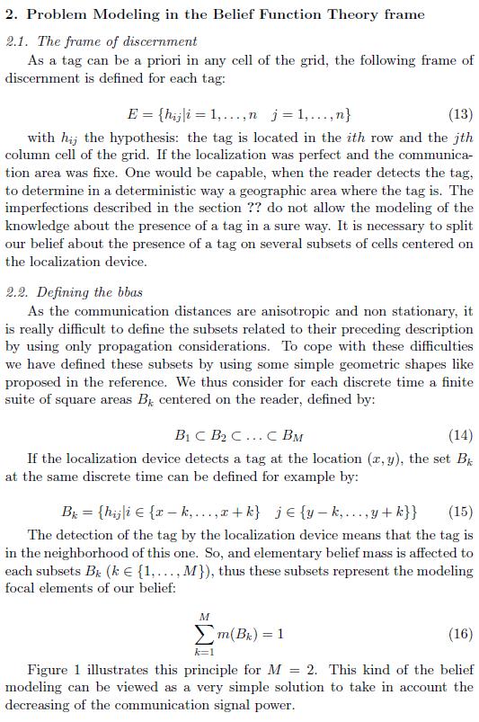
167 151

168 152

169 153

170 154

171 155

172 156

173 157

174 158

175 Appendix D Benefit Cost Model for RFID/GPS Based Automated Materials Tracking System Nasir conducted a cost-benefit analysis for RFID/GPS Based automated materials tracking system. This appendix is adopted from Nasir s Masters thesis (Nasir 2009): The fixed and variable cost of the system should be compared with the benefits that are expected to be provided by the system. These benefits can be direct benefits such as the number of man hours reduced for locating materials and reduction in lost labor hours due to otherwise delayed materials locating. The indirect benefits such as increase in productivity should also be considered. Estimates of indirect benefits and costs avoided may be based on simple risk analyses as described in the following section. Elements of the economic analysis include: Estimating the savings per standard locate reduced duration. Estimating the savings per temporary loss avoided. Estimating the savings per total loss and re-procurement avoided. Estimating benefits of expected improved productivity Total estimated cost for the system. Benefit/Cost ratio. Besides the above economic analysis, certain strategic analyses should also be considered such as repeatability or reuse of the design elements (once the initial investment is made, how much could be used again on future projects). For example the bar codes can be used for one time only, whereas the RFID tags are reusable. The life of RFID tags, the purchase of software or per year usage charges etc. should also be considered while evaluating the options. In the remainder of this section, an example of an analysis based on the preceding principles is presented with a typical industrial project in mind. Time value of money is not considered because of the project level planning horizon for the process described in this chapter. A benefit/cost analysis for a typical industrial project is presented in the following Table. This table provides the costs of active RFID tags, antennas, readers, GPS units, handheld PCs, and software required for the system. The costs are based on current average prices. It is assumed that the duration of the project will be 500 days and the 159

176 project will be an industrial one which involves thousands of high value engineered materials items such as spools, valves, steel members, turbines, and pumps etc. The project has vast scattered lay down yards, where the materials are frequently moved around before their final installation. Table D.1: Benefit Cost Model for RFID/GPS based automated materials tracking system 160

177 Three different scenarios are considered; scenario 1 being the least favourable situation where the least number of critical items are tagged, and the least expected number of materials locates are made per day, whereas scenario 3 represents the most favourable situation where the highest number of critical items are attached with tags and the expected number of locates per day is highest. The time saved per locate of items is based on the experience gained in the field trials at Portlands Energy Centre, Toronto, and Rockdale, Texas. The benefit cost ratios calculated as shown in the following table are without considering benefits of improved productivity and costs avoided due to reduced risk of lost and re-procured items. The savings or benefits are high compared to the total cost of the system. Therefore, the estimated benefit/cost ratios are also very high from worst to best case scenarios. Even in scenario 1, which is considered the least favourable situation, the B/C ratio suggests implementing the system on the typical project described. It is interesting that anecdotally, one major constructor on CII RT 240 estimated a B/C ratio of between 5/1 and 40/1, so it is possible that remaining benefits need to be considered. 161

178 Appendix E A Sample Subset of the Acquired Data from the Filed Experiment Figure E.1: Illustration of the data fields of a sample.kml file The following lines present a sample raw acquired data from the Portlands site in kml format. <kml xmlns:xsi=" xmlns:xsd=" xmlns=" <Document> <Placemark> <Point> <coordinates> , </coordinates> </Point> <name> </name> <Snippet maxlines="0">tag at 6/19/08 8:09:28 AM</Snippet> <description>tag located at 6/19/08 8:09:28 AM within 6.3 meters.</description> </Placemark> <Placemark> <Point> <coordinates> , </coordinates> </Point> <name> </name> <Snippet maxlines="0">tag at 6/19/08 8:11:18 AM</Snippet> <description>tag located at 6/19/08 8:11:18 AM within 7.0 meters.</description> </Placemark> <Placemark> 162